Deep Learning · MT2 · formulas
Output delta for half squared loss
Delta is a short name for the loss derivative with respect to a neuron’s raw input z. For half squared loss, multiply prediction minus target by the activation’s derivative. The result is then multiplied by an incoming activation to obtain a weight gradient.
 LaTeX:
\delta^{out}=(o-y)f\prime(z)Loss scaling: derive the gradient instead of guessing a factor
1. One error, three possible objectives
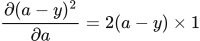
Let a be a prediction and y a fixed target. The error is a − y. The derivative of that error with respect to a is 1 because y stays fixed. Apply the chain rule to its square:
 LaTeX:
\frac{\partial (a-y)^2}{\partial a}=2(a-y)\times1Multiplying the objective by a constant multiplies its derivative by the same constant. This gives the common loss conventions below.
| Stated loss over n outputs | Derivative with respect to one prediction aⱼ |
|---|---|
| SSE: sum of all squared errors | 2(aⱼ − yⱼ) |
| Half SSE: half of that sum | aⱼ − yⱼ |
| MSE: that sum divided by n | 2(aⱼ − yⱼ)/n |
| Half MSE: that sum divided by 2n | (aⱼ − yⱼ)/n |
2. Why only the matching output appears
Suppose three predictions are separate output variables a₁, a₂ and a₃. When differentiating the loss with respect to a₂, the a₁ and a₃ terms are constant with respect to that output variable, so their direct derivatives are zero. The remaining term is the error of output 2, with the correct scaling factor.
Later, a shared hidden weight may influence all three predictions. Backpropagation then combines those separate output contributions through the chain rule. “Differentiate with respect to one output” and “differentiate with respect to a shared weight” are different stages.
3. The activation contributes another factor
If a = sigmoid(z), the derivative of a with respect to its input is a(1 − a). For half SSE, the output delta is therefore:
 LaTeX:
\delta=\frac{\partial L}{\partial z}=(a-y)a(1-a)For a linear output, the activation derivative is 1. For positive ReLU input it is also 1; for negative ReLU input it is 0. Always use the derivative of the activation actually given in the question.
4. A numerical comparison
For a = 0.7 and y = 1, the signed error is −0.3. For half SSE with sigmoid, the activation derivative is 0.7 × 0.3 = 0.21. The output delta is −0.3 × 0.21 = −0.063. With plain SSE it doubles to −0.126. With MSE over three outputs it is −0.126/3 = −0.042.
The forward prediction 0.7 did not change. The loss convention changed the gradient scale. This is why the first line of a backpropagation answer should state the loss being used.
Complete sigmoid training example
Question. A sigmoid neuron has input 2, weight 0, bias 0, target 1 and half squared loss. Will gradient descent increase or decrease the weight? Use learning rate 0.1 and calculate the exact update.
Given
x = 2; w = 0; b = 0; y = 1.
Sigmoid output; half squared loss; η = 0.1.
To find
Find the weight-gradient sign, exact weight update and resulting weight.
Formula — which one and why
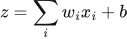
Weighted sum and activation. Each input is multiplied by its connection weight. Add these contributions, add the bias once, then apply the stated activation.
xᵢ = input i; wᵢ = its weight; b = bias; z = sum before activation; a = output after activation; f = the specified activation function.
 LaTeX:
z=\sum_iw_ix_i+b LaTeX:
a=f(z)Yaad rakhne ka cue: Input × weight, sabka sum, bias once, phir activation.
Sigmoid and its slope. Use sigmoid when the neuron is specified to squash its preactivation into (0,1). Once its output is known, its derivative needs only output × (1−output).
z = preactivation; p = sigmoid output; e is the exponential base, not a prediction error in this formula.
 LaTeX:
p=\frac{1}{1+e^{-z}}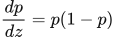 LaTeX:
\frac{dp}{dz}=p(1-p)Yaad rakhne ka cue: Sigmoid output p; uska slope p × (1−p).
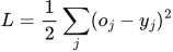
Half summed squared loss. This loss convention takes one-half of the sum of squared prediction errors. Use it when the question specifies it, or explicitly state it as an assumption when the paper omits the loss. Differentiating cancels the factor one-half against the square derivative.
oⱼ = output j; yⱼ = target j; L = half summed squared loss under the stated or explicitly assumed convention.
 LaTeX:
L=\frac12\sum_j(o_j-y_j)^2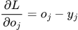 LaTeX:
\frac{\partial L}{\partial o_j}=o_j-y_jYaad rakhne ka cue: Half aur square ka 2 cancel: output derivative = prediction − target.
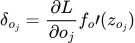
Backpropagation. The loss tells us how each output must change. Multiply by that neuron’s activation slope to obtain its delta. A weight gradient is receiving delta × sending value. Hidden deltas must include every outgoing path.
δ (delta) = derivative of loss with respect to a neuron’s preactivation; f′ = activation derivative; aᵢ = sending activation; Wⱼᵢ = connection weight. Use the exact loss scaling in the question.
 LaTeX:
\delta_{o_j}=\frac{\partial L}{\partial o_j}f_o\prime(z_{o_j})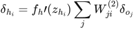 LaTeX:
\delta_{h_i}=f_h\prime(z_{h_i})\sum_jW_{ji}^{(2)}\delta_{o_j}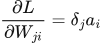 LaTeX:
\frac{\partial L}{\partial W_{ji}}=\delta_ja_i LaTeX:
\frac{\partial L}{\partial b_j}=\delta_j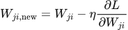 LaTeX:
W_{ji,\mathrm{new}}=W_{ji}-\eta\frac{\partial L}{\partial W_{ji}}Yaad rakhne ka cue: Receiving delta × sending value = us connection ka gradient.
Solution — step by step
Step 1 forward: net = 0(2) + 0 = 0; sigmoid output = 0.5.
Step 2 backward: prediction minus target = 0.5 − 1 = −0.5. Sigmoid slope = 0.5(1 − 0.5) = 0.25. Delta = −0.5 × 0.25 = −0.125.
Step 3 gradients and update: weight gradient = −0.125 × 2 = −0.25. New weight = 0 − 0.1(−0.25) = 0.025. Bias gradient = −0.125; new bias = 0.0125. Both increase. With positive input, these changes initially raise the prediction toward the target. Your intuition and arithmetic now agree.
Drill 10 Sigmoid neuron gradient
Question
Question. x = 2, w = 0.5, b = 0, y = 1, half squared loss, η = 0.1. Find one weight and bias update.
Answer — step by step
Given
x = 2; w = 0.5; b = 0; target y = 1.
Activation: sigmoid; loss: half squared error.
Learning rate η = 0.1.
To find
Find the output, delta, weight/bias gradients and one update.
Formula — which one and why
Weighted sum and activation. Each input is multiplied by its connection weight. Add these contributions, add the bias once, then apply the stated activation.
xᵢ = input i; wᵢ = its weight; b = bias; z = sum before activation; a = output after activation; f = the specified activation function.
LaTeX: z=\sum_iw_ix_i+bLaTeX: a=f(z)Yaad rakhne ka cue: Input × weight, sabka sum, bias once, phir activation.
Sigmoid and its slope. Use sigmoid when the neuron is specified to squash its preactivation into (0,1). Once its output is known, its derivative needs only output × (1−output).
z = preactivation; p = sigmoid output; e is the exponential base, not a prediction error in this formula.
LaTeX: p=\frac{1}{1+e^{-z}}LaTeX: \frac{dp}{dz}=p(1-p)Yaad rakhne ka cue: Sigmoid output p; uska slope p × (1−p).
Half summed squared loss. This loss convention takes one-half of the sum of squared prediction errors. Use it when the question specifies it, or explicitly state it as an assumption when the paper omits the loss. Differentiating cancels the factor one-half against the square derivative.
oⱼ = output j; yⱼ = target j; L = half summed squared loss under the stated or explicitly assumed convention.
LaTeX: L=\frac12\sum_j(o_j-y_j)^2LaTeX: \frac{\partial L}{\partial o_j}=o_j-y_jYaad rakhne ka cue: Half aur square ka 2 cancel: output derivative = prediction − target.
Backpropagation. The loss tells us how each output must change. Multiply by that neuron’s activation slope to obtain its delta. A weight gradient is receiving delta × sending value. Hidden deltas must include every outgoing path.
δ (delta) = derivative of loss with respect to a neuron’s preactivation; f′ = activation derivative; aᵢ = sending activation; Wⱼᵢ = connection weight. Use the exact loss scaling in the question.
LaTeX: \delta_{o_j}=\frac{\partial L}{\partial o_j}f_o\prime(z_{o_j})LaTeX: \delta_{h_i}=f_h\prime(z_{h_i})\sum_jW_{ji}^{(2)}\delta_{o_j}LaTeX: \frac{\partial L}{\partial W_{ji}}=\delta_ja_iLaTeX: \frac{\partial L}{\partial b_j}=\delta_jLaTeX: W_{ji,\mathrm{new}}=W_{ji}-\eta\frac{\partial L}{\partial W_{ji}}Yaad rakhne ka cue: Receiving delta × sending value = us connection ka gradient.
Solution — step by step
Meaning and formulas
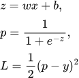
Here the loss is half squared error. It is different from binary cross-entropy, so we include the sigmoid derivative explicitly.
 LaTeX:
z=wx+b,\quad p=\frac1{1+e^{-z}},\quad L=\frac12(p-y)^2The symbol δ (delta) is a short name for the loss gradient with respect to the neuron's raw score z.
 LaTeX:
\delta=(p-y)p(1-p)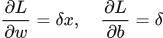 LaTeX:
\frac{\partial L}{\partial w}=\delta x,\quad \frac{\partial L}{\partial b}=\delta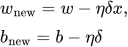 LaTeX:
w_{\mathrm{new}}=w-\eta\delta x,\quad b_{\mathrm{new}}=b-\eta\deltaStep 1: weighted sum and sigmoid
 LaTeX:
z=0.5\times2+0=1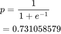 LaTeX:
p=\frac1{1+e^{-1}}=0.731058579Step 2: error and activation slope
 LaTeX:
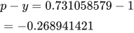
p-y=0.731058579-1=-0.268941421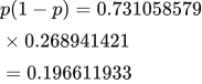 LaTeX:
p(1-p)=0.731058579\times0.268941421=0.196611933Step 3: multiply the linked effects to obtain delta
 LaTeX:
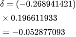
\delta=(-0.268941421)\times0.196611933=-0.052877093Step 4: multiply delta by the input to each parameter
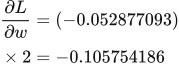
The weight receives x = 2. The bias effectively receives the constant input 1.
 LaTeX:
\frac{\partial L}{\partial w}=(-0.052877093)\times2=-0.105754186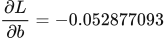 LaTeX:
\frac{\partial L}{\partial b}=-0.052877093Step 5: subtract learning rate times each gradient
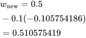 LaTeX:
w_{\mathrm{new}}=0.5-0.1(-0.105754186)=0.510575419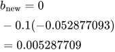 LaTeX:
b_{\mathrm{new}}=0-0.1(-0.052877093)=0.005287709Final answer: new weight ≈ 0.510575419; new bias ≈ 0.005287709. Subtracting negative gradients increases both values here.
Drill 11 Full ReLU backpropagation
Question
Question. Input x = [1, 2]. Each row below lists the incoming weights of one receiving neuron. W₁ is shown below; b₁ = [0.1, 0.2]; W₂ is shown below; b₂ = [0.1]. Hidden and output activations are ReLU. Target y = [1]. Learning rate η = 0.1. Use half squared loss and update all weights and biases.
Answer — step by step
Given
Input x = [1, 2].
W₁ is printed with the question.
b₁ = [0.1, 0.2].
W₂ is printed with the question.
b₂ = [0.1].
Hidden and output activations are ReLU.
Target y = [1].
Learning rate η = 0.1.
Use half squared loss and update all weights and biases.
To find
Find all preactivations, hidden activations and final outputs. Calculate the half summed squared loss and its output derivatives. Find the requested deltas and parameter gradients, then update the specified parameters.
Formula — which one and why
Forward propagation. Evaluate one layer completely before supplying its activated outputs to the next layer. Each layer has its own weights and biases.
x = input vector; h = hidden outputs; W₁,b₁ = hidden parameters; W₂,b₂ = output parameters; f₁,f₂ = the stated activations.
 LaTeX:
z_h=W_1x+b_1 LaTeX:
h=f_1(z_h) LaTeX:
z_o=W_2h+b_2 LaTeX:
o=f_2(z_o)Yaad rakhne ka cue: Pehli layer ka activated output hi agli layer ka input hai.
Half summed squared loss. This loss convention takes one-half of the sum of squared prediction errors. Use it when the question specifies it, or explicitly state it as an assumption when the paper omits the loss. Differentiating cancels the factor one-half against the square derivative.
oⱼ = output j; yⱼ = target j; L = half summed squared loss under the stated or explicitly assumed convention.
LaTeX: L=\frac12\sum_j(o_j-y_j)^2LaTeX: \frac{\partial L}{\partial o_j}=o_j-y_jYaad rakhne ka cue: Half aur square ka 2 cancel: output derivative = prediction − target.
Backpropagation. The loss tells us how each output must change. Multiply by that neuron’s activation slope to obtain its delta. A weight gradient is receiving delta × sending value. Hidden deltas must include every outgoing path.
δ (delta) = derivative of loss with respect to a neuron’s preactivation; f′ = activation derivative; aᵢ = sending activation; Wⱼᵢ = connection weight. Use the exact loss scaling in the question.
LaTeX: \delta_{o_j}=\frac{\partial L}{\partial o_j}f_o\prime(z_{o_j})LaTeX: \delta_{h_i}=f_h\prime(z_{h_i})\sum_jW_{ji}^{(2)}\delta_{o_j}LaTeX: \frac{\partial L}{\partial W_{ji}}=\delta_ja_iLaTeX: \frac{\partial L}{\partial b_j}=\delta_jLaTeX: W_{ji,\mathrm{new}}=W_{ji}-\eta\frac{\partial L}{\partial W_{ji}}Yaad rakhne ka cue: Receiving delta × sending value = us connection ka gradient.
Solution — step by step
Formulas used before substituting numbers
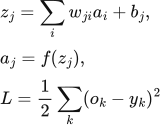
For every receiving neuron, z is its weighted sum and a is its activated output. The half squared loss sums the errors from all output neurons.
 LaTeX:
z_j=\sum_iw_{ji}a_i+b_j,\quad a_j=f(z_j),\quad L=\frac12\sum_k(o_k-y_k)^2Delta means the loss gradient with respect to a neuron's raw score. First calculate output deltas, then hidden deltas using every connected output path.
 LaTeX:
\delta_{o_k}=(o_k-y_k)f'(z_{o_k})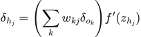 LaTeX:
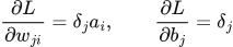
\delta_{h_j}=\left(\sum_kw_{kj}\delta_{o_k}\right)f'(z_{h_j})The gradient of a connection is its receiving delta multiplied by its sending activation. A bias receives the constant 1.
 LaTeX:
\frac{\partial L}{\partial w_{ji}}=\delta_j a_i,\qquad \frac{\partial L}{\partial b_j}=\delta_j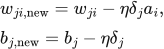 LaTeX:
w_{ji,\mathrm{new}}=w_{ji}-\eta\delta_j a_i,\quad b_{j,\mathrm{new}}=b_j-\eta\delta_jFor sigmoid, use f′ = a(1 − a). For ReLU, use f′ = 1 for a positive raw score and 0 for a negative raw score. Store the old weights until all gradients have been calculated.
Step 1 map the arrows. Each row of W₁ receives all inputs; each row of W₂ receives all hidden outputs. Bias is added once per receiving neuron. All gradients below use the OLD weights from this same forward pass.
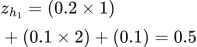
Hidden neuron 1:
 LaTeX:
z_{h_1} = (0.2 \times 1) + (0.1 \times 2) + (0.1) = 0.5 LaTeX:
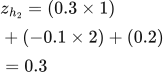
h_{1} = \max(0,0.5) = 0.5Hidden neuron 2:
 LaTeX:
z_{h_2} = (0.3 \times 1) + (-0.1 \times 2) + (0.2) = 0.3 LaTeX:
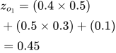
h_{2} = \max(0,0.3) = 0.3Output neuron 1:
 LaTeX:
z_{o_1} = (0.4 \times 0.5) + (0.5 \times 0.3) + (0.1) = 0.45 LaTeX:
o_{1} = \max(0,0.45) = 0.45Step 2 loss convention. This worked solution uses half summed squared loss, L = ½Σ(o − y)². Follow the loss specified in the question; where none is supplied, this is an explicit assumption.
Prediction minus target = [-0.55]. Squared errors = [0.3025]. Half-sum squared loss = 0.15125; mean squared error = 0.3025. These are different unless the number of output components makes the scale coincide.
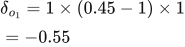
Output delta 1:
 LaTeX:
\delta_{o_1} = 1 \times (0.45-1) \times 1 = -0.55The ReLU derivative is 1 here because this preactivation is positive.
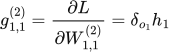
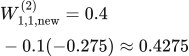
Step 3 output weights. Gradient = receiving delta × sending activation. An output bias gradient equals its delta.
h1 → o1:
Subtract η × gradient = −0.0275. This weight increases.
The sending value and receiving delta have different roles. All deltas still use the original forward-pass weights.
The receiving neuron supplies the delta; the sending neuron supplies its activation.
 LaTeX:
g_{1,1}^{(2)}=\frac{\partial L}{\partial W^{(2)}_{1,1}}=\delta_{o_1}h_1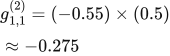 LaTeX:
g_{1,1}^{(2)}=(-0.55)\times(0.5)\approx -0.275Apply the learning rate to this gradient and subtract the result from the old weight.
 LaTeX:
W^{(2)}_{1,1,\mathrm{new}}=0.4-0.1(-0.275)\approx 0.4275h2 → o1:
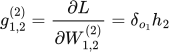
Subtract η × gradient = −0.0165. This weight increases.
The sending value and receiving delta have different roles. All deltas still use the original forward-pass weights.
The receiving neuron supplies the delta; the sending neuron supplies its activation.
 LaTeX:
g_{1,2}^{(2)}=\frac{\partial L}{\partial W^{(2)}_{1,2}}=\delta_{o_1}h_2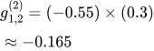 LaTeX:
g_{1,2}^{(2)}=(-0.55)\times(0.3)\approx -0.165Apply the learning rate to this gradient and subtract the result from the old weight.
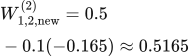 LaTeX:
W^{(2)}_{1,2,\mathrm{new}}=0.5-0.1(-0.165)\approx 0.5165Step 4 hidden deltas. A hidden unit can influence EVERY connected output, so add those paths BEFORE multiplying by the hidden activation derivative.
Hidden 1 downstream contribution:
Calculate each outgoing path using the old outgoing weight and that output's delta.
Multiply within each path. Add the resulting contributions at the shared hidden neuron.
Contribution from output 1.
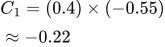 LaTeX:
C_1=(0.4)\times(-0.55)\approx -0.22Accumulate the contributions, then apply the hidden activation derivative below.
 LaTeX:
\text{Sum}=C_1\approx -0.22 LaTeX:
\delta_{h_1} = -0.22 \times 1 = -0.22Hidden 2 downstream contribution:
Calculate each outgoing path using the old outgoing weight and that output's delta.
Multiply within each path. Add the resulting contributions at the shared hidden neuron.
Contribution from output 1.
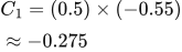 LaTeX:
C_1=(0.5)\times(-0.55)\approx -0.275Accumulate the contributions, then apply the hidden activation derivative below.
 LaTeX:
\text{Sum}=C_1\approx -0.275 LaTeX:
\delta_{h_2} = -0.275 \times 1 = -0.275Step 5 input weights. Multiply the hidden delta by the corresponding raw input, not by the hidden output.
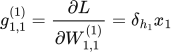
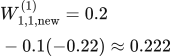
x1 → h1:
Subtract η × gradient = −0.022. This weight increases.
The sending value and receiving delta have different roles. All deltas still use the original forward-pass weights.
The receiving neuron supplies the delta; the sending neuron supplies the input value.
 LaTeX:
g_{1,1}^{(1)}=\frac{\partial L}{\partial W^{(1)}_{1,1}}=\delta_{h_1}x_1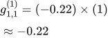 LaTeX:
g_{1,1}^{(1)}=(-0.22)\times(1)\approx -0.22Apply the learning rate to this gradient and subtract the result from the old weight.
 LaTeX:
W^{(1)}_{1,1,\mathrm{new}}=0.2-0.1(-0.22)\approx 0.222x2 → h1:
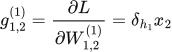
Subtract η × gradient = −0.044. This weight increases.
The sending value and receiving delta have different roles. All deltas still use the original forward-pass weights.
The receiving neuron supplies the delta; the sending neuron supplies the input value.
 LaTeX:
g_{1,2}^{(1)}=\frac{\partial L}{\partial W^{(1)}_{1,2}}=\delta_{h_1}x_2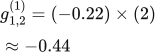 LaTeX:
g_{1,2}^{(1)}=(-0.22)\times(2)\approx -0.44Apply the learning rate to this gradient and subtract the result from the old weight.
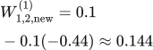 LaTeX:
W^{(1)}_{1,2,\mathrm{new}}=0.1-0.1(-0.44)\approx 0.144x1 → h2:
Subtract η × gradient = −0.0275. This weight increases.
The sending value and receiving delta have different roles. All deltas still use the original forward-pass weights.
The receiving neuron supplies the delta; the sending neuron supplies the input value.
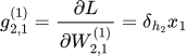 LaTeX:
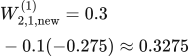
g_{2,1}^{(1)}=\frac{\partial L}{\partial W^{(1)}_{2,1}}=\delta_{h_2}x_1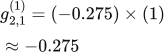 LaTeX:
g_{2,1}^{(1)}=(-0.275)\times(1)\approx -0.275Apply the learning rate to this gradient and subtract the result from the old weight.
 LaTeX:
W^{(1)}_{2,1,\mathrm{new}}=0.3-0.1(-0.275)\approx 0.3275x2 → h2:
Subtract η × gradient = −0.055. This weight increases.
The sending value and receiving delta have different roles. All deltas still use the original forward-pass weights.
The receiving neuron supplies the delta; the sending neuron supplies the input value.
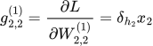 LaTeX:
g_{2,2}^{(1)}=\frac{\partial L}{\partial W^{(1)}_{2,2}}=\delta_{h_2}x_2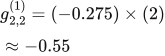 LaTeX:
g_{2,2}^{(1)}=(-0.275)\times(2)\approx -0.55Apply the learning rate to this gradient and subtract the result from the old weight.
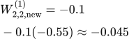 LaTeX:
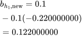
W^{(1)}_{2,2,\mathrm{new}}=-0.1-0.1(-0.55)\approx -0.045Step 6 bias updates. A bias receives a constant input 1, so its gradient equals the corresponding delta. Use the same old forward pass and learning rate as the weight updates.
 LaTeX:
b_{h_1,\mathrm{new}}=0.1-0.1(-0.220000000)=0.122000000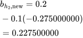 LaTeX:
b_{h_2,\mathrm{new}}=0.2-0.1(-0.275000000)=0.227500000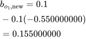 LaTeX:
b_{o_1,\mathrm{new}}=0.1-0.1(-0.550000000)=0.155000000These are independent per-neuron biases. If the question fixes biases, keep them fixed. If it specifies a single tied bias, add all deltas sharing that bias before updating it.
Drill 12 Two output sigmoid backpropagation
Question
Question. Input x = [0.2, 0.4]. Each row below lists the incoming weights of one receiving neuron. W₁ is shown below; b₁ = [0.1, 0.1]; W₂ is shown below; b₂ = [0, 0.1]. Hidden and output activations are sigmoid. Target y = [1, 0]. Learning rate η = 0.2. Use half summed squared loss and update all parameters.
Answer — step by step
Given
Input x = [0.2, 0.4].
W₁ is printed with the question.
b₁ = [0.1, 0.1].
W₂ is printed with the question.
b₂ = [0, 0.1].
Hidden and output activations are sigmoid.
Target y = [1, 0].
Learning rate η = 0.2.
Use half summed squared loss and update all parameters.
To find
Find all preactivations, hidden activations and final outputs. Calculate the half summed squared loss and its output derivatives. Find the sigmoid output and, if requested, its derivative. Find the requested deltas and parameter gradients, then update the specified parameters.
Formula — which one and why
Forward propagation. Evaluate one layer completely before supplying its activated outputs to the next layer. Each layer has its own weights and biases.
x = input vector; h = hidden outputs; W₁,b₁ = hidden parameters; W₂,b₂ = output parameters; f₁,f₂ = the stated activations.
LaTeX: z_h=W_1x+b_1LaTeX: h=f_1(z_h)LaTeX: z_o=W_2h+b_2LaTeX: o=f_2(z_o)Yaad rakhne ka cue: Pehli layer ka activated output hi agli layer ka input hai.
Half summed squared loss. This loss convention takes one-half of the sum of squared prediction errors. Use it when the question specifies it, or explicitly state it as an assumption when the paper omits the loss. Differentiating cancels the factor one-half against the square derivative.
oⱼ = output j; yⱼ = target j; L = half summed squared loss under the stated or explicitly assumed convention.
LaTeX: L=\frac12\sum_j(o_j-y_j)^2LaTeX: \frac{\partial L}{\partial o_j}=o_j-y_jYaad rakhne ka cue: Half aur square ka 2 cancel: output derivative = prediction − target.
Sigmoid and its slope. Use sigmoid when the neuron is specified to squash its preactivation into (0,1). Once its output is known, its derivative needs only output × (1−output).
z = preactivation; p = sigmoid output; e is the exponential base, not a prediction error in this formula.
LaTeX: p=\frac{1}{1+e^{-z}}LaTeX: \frac{dp}{dz}=p(1-p)Yaad rakhne ka cue: Sigmoid output p; uska slope p × (1−p).
Backpropagation. The loss tells us how each output must change. Multiply by that neuron’s activation slope to obtain its delta. A weight gradient is receiving delta × sending value. Hidden deltas must include every outgoing path.
δ (delta) = derivative of loss with respect to a neuron’s preactivation; f′ = activation derivative; aᵢ = sending activation; Wⱼᵢ = connection weight. Use the exact loss scaling in the question.
LaTeX: \delta_{o_j}=\frac{\partial L}{\partial o_j}f_o\prime(z_{o_j})LaTeX: \delta_{h_i}=f_h\prime(z_{h_i})\sum_jW_{ji}^{(2)}\delta_{o_j}LaTeX: \frac{\partial L}{\partial W_{ji}}=\delta_ja_iLaTeX: \frac{\partial L}{\partial b_j}=\delta_jLaTeX: W_{ji,\mathrm{new}}=W_{ji}-\eta\frac{\partial L}{\partial W_{ji}}Yaad rakhne ka cue: Receiving delta × sending value = us connection ka gradient.
Solution — step by step
Formulas used before substituting numbers
For every receiving neuron, z is its weighted sum and a is its activated output. The half squared loss sums the errors from all output neurons.
LaTeX: z_j=\sum_iw_{ji}a_i+b_j,\quad a_j=f(z_j),\quad L=\frac12\sum_k(o_k-y_k)^2Delta means the loss gradient with respect to a neuron's raw score. First calculate output deltas, then hidden deltas using every connected output path.
LaTeX: \delta_{o_k}=(o_k-y_k)f'(z_{o_k})LaTeX: \delta_{h_j}=\left(\sum_kw_{kj}\delta_{o_k}\right)f'(z_{h_j})The gradient of a connection is its receiving delta multiplied by its sending activation. A bias receives the constant 1.
LaTeX: \frac{\partial L}{\partial w_{ji}}=\delta_j a_i,\qquad \frac{\partial L}{\partial b_j}=\delta_jLaTeX: w_{ji,\mathrm{new}}=w_{ji}-\eta\delta_j a_i,\quad b_{j,\mathrm{new}}=b_j-\eta\delta_jFor sigmoid, use f′ = a(1 − a). For ReLU, use f′ = 1 for a positive raw score and 0 for a negative raw score. Store the old weights until all gradients have been calculated.
Step 1 map the arrows. Each row of W₁ receives all inputs; each row of W₂ receives all hidden outputs. Bias is added once per receiving neuron. All gradients below use the OLD weights from this same forward pass.
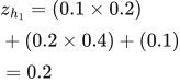
Hidden neuron 1:
 LaTeX:
z_{h_1} = (0.1 \times 0.2) + (0.2 \times 0.4) + (0.1) = 0.2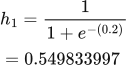 LaTeX:
h_{1}=\frac{1}{1+e^{-(0.2)}}=0.549833997Hidden neuron 2:
 LaTeX:
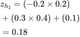
z_{h_2} = (-0.2 \times 0.2) + (0.3 \times 0.4) + (0.1) = 0.18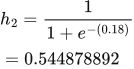 LaTeX:
h_{2}=\frac{1}{1+e^{-(0.18)}}=0.544878892Output neuron 1:
 LaTeX:
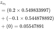
z_{o_1} = (0.2 \times 0.549833997) + (-0.1 \times 0.544878892) + (0) = 0.05547891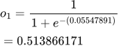 LaTeX:
o_{1}=\frac{1}{1+e^{-(0.05547891)}}=0.513866171Output neuron 2:
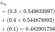 LaTeX:
z_{o_2} = (0.3 \times 0.549833997) + (0.4 \times 0.544878892) + (0.1) = 0.482901756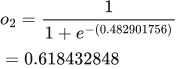 LaTeX:
o_{2}=\frac{1}{1+e^{-(0.482901756)}}=0.618432848Step 2 loss convention. This worked solution uses half summed squared loss, L = ½Σ(o − y)². Follow the loss specified in the question; where none is supplied, this is an explicit assumption.
Prediction minus target = [-0.486133829, 0.618432848]. Squared errors = [0.2363261, 0.382459187]. Half-sum squared loss = 0.309392643; mean squared error = 0.309392643. These are different unless the number of output components makes the scale coincide.
Output delta 1:
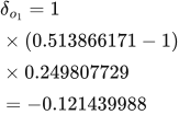 LaTeX:
\delta_{o_1} = 1 \times (0.513866171-1) \times 0.249807729 = -0.121439988The derivative is o(1−o).
Output delta 2:
 LaTeX:
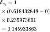
\delta_{o_2} = 1 \times (0.618432848-0) \times 0.235973661 = 0.145933863The derivative is o(1−o).
Step 3 output weights. Gradient = receiving delta × sending activation. An output bias gradient equals its delta.
h1 → o1:
Subtract η × gradient = −0.013354367. This weight increases.
The sending value and receiving delta have different roles. All deltas still use the original forward-pass weights.
The receiving neuron supplies the delta; the sending neuron supplies its activation.
LaTeX: g_{1,1}^{(2)}=\frac{\partial L}{\partial W^{(2)}_{1,1}}=\delta_{o_1}h_1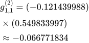 LaTeX:
g_{1,1}^{(2)}=(-0.121439988)\times(0.549833997)\approx -0.066771834Apply the learning rate to this gradient and subtract the result from the old weight.
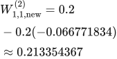 LaTeX:
W^{(2)}_{1,1,\mathrm{new}}=0.2-0.2(-0.066771834)\approx 0.213354367h2 → o1:
Subtract η × gradient = −0.013234017. This weight increases.
The sending value and receiving delta have different roles. All deltas still use the original forward-pass weights.
The receiving neuron supplies the delta; the sending neuron supplies its activation.
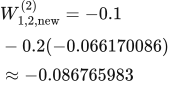
LaTeX: g_{1,2}^{(2)}=\frac{\partial L}{\partial W^{(2)}_{1,2}}=\delta_{o_1}h_2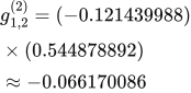 LaTeX:
g_{1,2}^{(2)}=(-0.121439988)\times(0.544878892)\approx -0.066170086Apply the learning rate to this gradient and subtract the result from the old weight.
 LaTeX:
W^{(2)}_{1,2,\mathrm{new}}=-0.1-0.2(-0.066170086)\approx -0.086765983h1 → o2:
Subtract η × gradient = 0.01604788. This weight decreases.
The sending value and receiving delta have different roles. All deltas still use the original forward-pass weights.
The receiving neuron supplies the delta; the sending neuron supplies its activation.
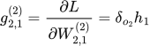 LaTeX:
g_{2,1}^{(2)}=\frac{\partial L}{\partial W^{(2)}_{2,1}}=\delta_{o_2}h_1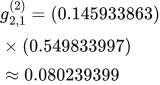 LaTeX:
g_{2,1}^{(2)}=(0.145933863)\times(0.549833997)\approx 0.080239399Apply the learning rate to this gradient and subtract the result from the old weight.
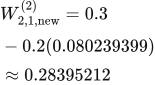 LaTeX:
W^{(2)}_{2,1,\mathrm{new}}=0.3-0.2(0.080239399)\approx 0.28395212h2 → o2:
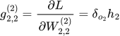
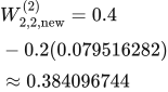
Subtract η × gradient = 0.015903256. This weight decreases.
The sending value and receiving delta have different roles. All deltas still use the original forward-pass weights.
The receiving neuron supplies the delta; the sending neuron supplies its activation.
 LaTeX:
g_{2,2}^{(2)}=\frac{\partial L}{\partial W^{(2)}_{2,2}}=\delta_{o_2}h_2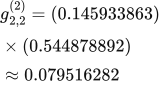 LaTeX:
g_{2,2}^{(2)}=(0.145933863)\times(0.544878892)\approx 0.079516282Apply the learning rate to this gradient and subtract the result from the old weight.
 LaTeX:
W^{(2)}_{2,2,\mathrm{new}}=0.4-0.2(0.079516282)\approx 0.384096744Step 4 hidden deltas. A hidden unit can influence EVERY connected output, so add those paths BEFORE multiplying by the hidden activation derivative.
Hidden 1 downstream contribution:
Calculate each outgoing path using the old outgoing weight and that output's delta.
Multiply within each path. Add the resulting contributions at the shared hidden neuron.
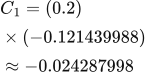
Contribution from output 1.
 LaTeX:
C_1=(0.2)\times(-0.121439988)\approx -0.024287998Contribution from output 2.
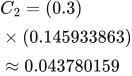 LaTeX:
C_2=(0.3)\times(0.145933863)\approx 0.043780159Accumulate the contributions, then apply the hidden activation derivative below.
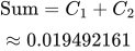 LaTeX:
\text{Sum}=C_1+C_2\approx 0.019492161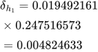 LaTeX:
\delta_{h_1} = 0.019492161 \times 0.247516573 = 0.004824633Hidden 2 downstream contribution:
Calculate each outgoing path using the old outgoing weight and that output's delta.
Multiply within each path. Add the resulting contributions at the shared hidden neuron.
Contribution from output 1.
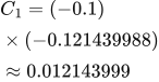 LaTeX:
C_1=(-0.1)\times(-0.121439988)\approx 0.012143999Contribution from output 2.
 LaTeX:
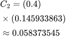
C_2=(0.4)\times(0.145933863)\approx 0.058373545Accumulate the contributions, then apply the hidden activation derivative below.
 LaTeX:
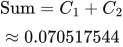
\text{Sum}=C_1+C_2\approx 0.070517544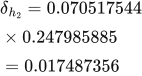 LaTeX:
\delta_{h_2} = 0.070517544 \times 0.247985885 = 0.017487356Step 5 input weights. Multiply the hidden delta by the corresponding raw input, not by the hidden output.
x1 → h1:
Subtract η × gradient = 0.000192985. This weight decreases.
The sending value and receiving delta have different roles. All deltas still use the original forward-pass weights.
The receiving neuron supplies the delta; the sending neuron supplies the input value.
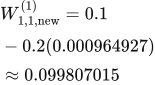
LaTeX: g_{1,1}^{(1)}=\frac{\partial L}{\partial W^{(1)}_{1,1}}=\delta_{h_1}x_1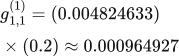 LaTeX:
g_{1,1}^{(1)}=(0.004824633)\times(0.2)\approx 0.000964927Apply the learning rate to this gradient and subtract the result from the old weight.
 LaTeX:
W^{(1)}_{1,1,\mathrm{new}}=0.1-0.2(0.000964927)\approx 0.099807015x2 → h1:
Subtract η × gradient = 0.000385971. This weight decreases.
The sending value and receiving delta have different roles. All deltas still use the original forward-pass weights.
The receiving neuron supplies the delta; the sending neuron supplies the input value.
LaTeX: g_{1,2}^{(1)}=\frac{\partial L}{\partial W^{(1)}_{1,2}}=\delta_{h_1}x_2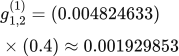 LaTeX:
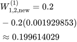
g_{1,2}^{(1)}=(0.004824633)\times(0.4)\approx 0.001929853Apply the learning rate to this gradient and subtract the result from the old weight.
 LaTeX:
W^{(1)}_{1,2,\mathrm{new}}=0.2-0.2(0.001929853)\approx 0.199614029x1 → h2:
Subtract η × gradient = 0.000699494. This weight decreases.
The sending value and receiving delta have different roles. All deltas still use the original forward-pass weights.
The receiving neuron supplies the delta; the sending neuron supplies the input value.
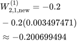
LaTeX: g_{2,1}^{(1)}=\frac{\partial L}{\partial W^{(1)}_{2,1}}=\delta_{h_2}x_1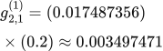 LaTeX:
g_{2,1}^{(1)}=(0.017487356)\times(0.2)\approx 0.003497471Apply the learning rate to this gradient and subtract the result from the old weight.
 LaTeX:
W^{(1)}_{2,1,\mathrm{new}}=-0.2-0.2(0.003497471)\approx -0.200699494x2 → h2:
Subtract η × gradient = 0.001398988. This weight decreases.
The sending value and receiving delta have different roles. All deltas still use the original forward-pass weights.
The receiving neuron supplies the delta; the sending neuron supplies the input value.
LaTeX: g_{2,2}^{(1)}=\frac{\partial L}{\partial W^{(1)}_{2,2}}=\delta_{h_2}x_2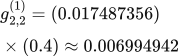 LaTeX:
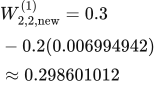
g_{2,2}^{(1)}=(0.017487356)\times(0.4)\approx 0.006994942Apply the learning rate to this gradient and subtract the result from the old weight.
 LaTeX:
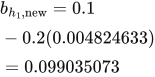
W^{(1)}_{2,2,\mathrm{new}}=0.3-0.2(0.006994942)\approx 0.298601012Step 6 bias updates. A bias receives a constant input 1, so its gradient equals the corresponding delta. Use the same old forward pass and learning rate as the weight updates.
 LaTeX:
b_{h_1,\mathrm{new}}=0.1-0.2(0.004824633)=0.099035073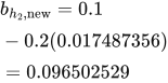 LaTeX:
b_{h_2,\mathrm{new}}=0.1-0.2(0.017487356)=0.096502529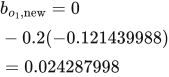 LaTeX:
b_{o_1,\mathrm{new}}=0-0.2(-0.121439988)=0.024287998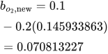 LaTeX:
b_{o_2,\mathrm{new}}=0.1-0.2(0.145933863)=0.070813227These are independent per-neuron biases. If the question fixes biases, keep them fixed. If it specifies a single tied bias, add all deltas sharing that bias before updating it.