Deep Learning · MT2 · formulas
Hidden delta, weight gradient and bias gradient
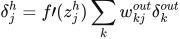
A hidden neuron can influence several outputs. Add all those backward contributions before multiplying by its own activation derivative. For each connection, use the receiving neuron’s delta and the sending neuron’s activation. Keep the old weights unchanged until all gradients have been found.
 LaTeX:
\delta_j^h=f\prime(z_j^h)\sum_k w_{kj}^{out}\delta_k^{out} LaTeX:
\frac{\partial L}{\partial w_{ji}}=\delta_j a_i LaTeX:
\frac{\partial L}{\partial b_j}=\delta_jMore outputs and vectorized backpropagation
Definition. Vectorized backpropagation expresses the chain rule using matrix products and elementwise derivatives. When a hidden activation affects several outputs, its derivative contains the sum of the contributions from every downstream path.
Why the hidden derivative is a sum
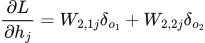
If hidden activation hⱼ connects to output preactivations zₒ₁ and zₒ₂, changing hⱼ changes both outputs. The multivariable chain rule gives:
 LaTeX:
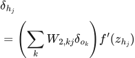
\frac{\partial L}{\partial h_j}=W_{2,1j}\delta_{o_1}+W_{2,2j}\delta_{o_2}For any number of connected outputs, sum their contributions and then differentiate the hidden activation:
 LaTeX:
\delta_{h_j}=\left(\sum_k W_{2,kj}\delta_{o_k}\right)f'(z_{h_j})Use the connecting weights from the original forward pass. Adding only the contribution of the first output would omit a dependency of the loss.
Matrix equations for one training sample
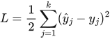
Use column vectors throughout. Let W₁ map d inputs to m hidden units and W₂ map those units to k outputs. The following output-delta formula assumes half sum of squared errors and an elementwise output activation f₂:
 LaTeX:
L=\frac12\sum_{j=1}^{k}(\hat y_j-y_j)^2 LaTeX:
\delta_2=(\hat y-y)\odot f_2'(z_2)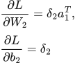 LaTeX:
\frac{\partial L}{\partial W_2}=\delta_2a_1^T,\qquad\frac{\partial L}{\partial b_2}=\delta_2 LaTeX:
\delta_1=(W_2^T\delta_2)\odot f_1'(z_1)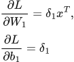 LaTeX:
\frac{\partial L}{\partial W_1}=\delta_1x^T,\qquad\frac{\partial L}{\partial b_1}=\delta_1Here ⊙ means elementwise multiplication. The product δ₂a₁ᵀ is an outer product: every receiving delta is multiplied by every sending activation.
| Quantity | Shape | Reason |
|---|---|---|
| W₁ and its gradient | m × d | m receiving hidden neurons, d inputs |
| W₂ and its gradient | k × m | k receiving output neurons, m hidden activations |
| δ₂ | k × 1 | One derivative per output preactivation |
| W₂ᵀδ₂ | m × 1 | The summed downstream derivative for each hidden unit |
| δ₂a₁ᵀ | (k × 1)(1 × m) = k × m | The output-weight gradient has the same shape as W₂ |
How the loss changes the output delta
For MSE averaged over k output components, the squared-error derivative has the factor 2/k. For sigmoid with binary cross-entropy, or softmax with categorical cross-entropy and a normalized target, the paired derivative simplifies to prediction minus target:
 LaTeX:
\delta_{\mathrm{output}}=\hat y-yThat simplification already includes differentiation of the paired activation and loss. Multiplying by a sigmoid derivative again would be incorrect. For sigmoid with half squared error, the sigmoid derivative is still required.
For a batch, sum per-example parameter gradients; divide by the batch size only if the objective is a batch mean. State the output reduction and batch reduction separately when both appear in a question.
Backpropagation with one hidden neuron
Definition. Backpropagation computes the derivatives of a scalar objective with respect to network parameters by applying the chain rule in reverse through the computational graph. An optimizer then uses these derivatives to update the parameters.
Network equations and the meaning of delta
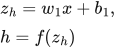
Consider one input, one hidden neuron and one output neuron:
 LaTeX:
z_h=w_1x+b_1,\qquad h=f(z_h)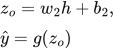 LaTeX:
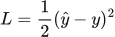
z_o=w_2h+b_2,\qquad\hat y=g(z_o)For the half squared loss used in this example:
 LaTeX:
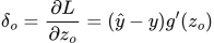
L=\frac12(\hat y-y)^2Define a neuron's delta as the derivative of the loss with respect to its preactivation, not with respect to its output:
 LaTeX:
\delta_o=\frac{\partial L}{\partial z_o}=(\hat y-y)g'(z_o)The output-weight derivative contains the hidden activation because zₒ = w₂h + b₂:
 LaTeX:
\frac{\partial L}{\partial w_2}=\delta_o h,\qquad\frac{\partial L}{\partial b_2}=\delta_oTo reach the hidden neuron, continue backwards through the old output weight and the hidden activation:
 LaTeX:
\delta_h=\delta_o w_2 f'(z_h) LaTeX:
\frac{\partial L}{\partial w_1}=\delta_h x,\qquad\frac{\partial L}{\partial b_1}=\delta_hThe bias derivative equals the corresponding delta because the derivative of z with respect to its additive bias is 1. All these derivatives belong to the same forward pass; an updated weight must not be used partway through this backward pass.
Complete worked numerical
Question. x = 2, y = 1; w₁ = 0.5, b₁ = 0.1; w₂ = 0.8, b₂ = 0.2. Both neurons use ReLU. Use half squared loss. Find the output and all four parameter gradients, then update all four parameters using η = 0.1.
Given
x = 2, y = 1.
w₁ = 0.5, b₁ = 0.1.
w₂ = 0.8, b₂ = 0.2.
Both neurons use ReLU.
Use half squared loss.
Find the output and all four parameter gradients, then update all four parameters using η = 0.1.
To find
Find all preactivations, hidden activations and final outputs. Calculate the half summed squared loss and its output derivatives. Find the requested deltas and parameter gradients, then update the specified parameters.
Formula — which one and why
Forward propagation. Evaluate one layer completely before supplying its activated outputs to the next layer. Each layer has its own weights and biases.
x = input vector; h = hidden outputs; W₁,b₁ = hidden parameters; W₂,b₂ = output parameters; f₁,f₂ = the stated activations.
 LaTeX:
z_h=W_1x+b_1 LaTeX:
h=f_1(z_h) LaTeX:
z_o=W_2h+b_2 LaTeX:
o=f_2(z_o)Yaad rakhne ka cue: Pehli layer ka activated output hi agli layer ka input hai.
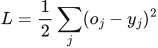
Half summed squared loss. This loss convention takes one-half of the sum of squared prediction errors. Use it when the question specifies it, or explicitly state it as an assumption when the paper omits the loss. Differentiating cancels the factor one-half against the square derivative.
oⱼ = output j; yⱼ = target j; L = half summed squared loss under the stated or explicitly assumed convention.
 LaTeX:
L=\frac12\sum_j(o_j-y_j)^2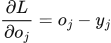 LaTeX:
\frac{\partial L}{\partial o_j}=o_j-y_jYaad rakhne ka cue: Half aur square ka 2 cancel: output derivative = prediction − target.
Backpropagation. The loss tells us how each output must change. Multiply by that neuron’s activation slope to obtain its delta. A weight gradient is receiving delta × sending value. Hidden deltas must include every outgoing path.
δ (delta) = derivative of loss with respect to a neuron’s preactivation; f′ = activation derivative; aᵢ = sending activation; Wⱼᵢ = connection weight. Use the exact loss scaling in the question.
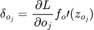 LaTeX:
\delta_{o_j}=\frac{\partial L}{\partial o_j}f_o\prime(z_{o_j})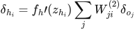 LaTeX:
\delta_{h_i}=f_h\prime(z_{h_i})\sum_jW_{ji}^{(2)}\delta_{o_j}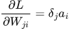 LaTeX:
\frac{\partial L}{\partial W_{ji}}=\delta_ja_iLaTeX: \frac{\partial L}{\partial b_j}=\delta_j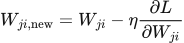 LaTeX:
W_{ji,\mathrm{new}}=W_{ji}-\eta\frac{\partial L}{\partial W_{ji}}Yaad rakhne ka cue: Receiving delta × sending value = us connection ka gradient.
Solution — step by step
Step 1: forward propagation through the hidden neuron.
 LaTeX:
z_h=0.5(2)+0.1=1.1 LaTeX:
h=\operatorname{ReLU}(1.1)=1.1Step 2: forward propagation through the output neuron.
 LaTeX:
z_o=0.8(1.1)+0.2=1.08 LaTeX:
\hat y=\operatorname{ReLU}(1.08)=1.08ReLU is not bounded above by 1, so this output is valid. It is not being interpreted as a probability here.
Step 3: calculate the loss and output delta.
 LaTeX:
L=\frac12(1.08-1)^2=0.0032Both preactivations are positive, so both ReLU derivatives are 1.
 LaTeX:
\delta_o=(1.08-1)(1)=0.08Step 4: calculate the output-layer parameter gradients.
 LaTeX:
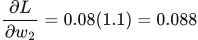
\frac{\partial L}{\partial w_2}=0.08(1.1)=0.088 LaTeX:
\frac{\partial L}{\partial b_2}=0.08Step 5: propagate the derivative to the hidden neuron.
Use w₂ = 0.8, its value during the forward pass:
 LaTeX:
\delta_h=0.08(0.8)(1)=0.064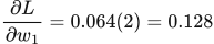 LaTeX:
\frac{\partial L}{\partial w_1}=0.064(2)=0.128 LaTeX:
\frac{\partial L}{\partial b_1}=0.064Step 6: update each parameter using its own gradient.
 LaTeX:
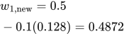
w_{1,\mathrm{new}}=0.5-0.1(0.128)=0.4872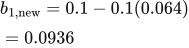 LaTeX:
b_{1,\mathrm{new}}=0.1-0.1(0.064)=0.0936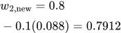 LaTeX:
w_{2,\mathrm{new}}=0.8-0.1(0.088)=0.7912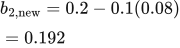 LaTeX:
b_{2,\mathrm{new}}=0.2-0.1(0.08)=0.192| Parameter | Gradient from the original forward pass | Updated value |
|---|---|---|
| w₁ | 0.128 | 0.4872 |
| b₁ | 0.064 | 0.0936 |
| w₂ | 0.088 | 0.7912 |
| b₂ | 0.08 | 0.192 |
Final answer: the original prediction is 1.08 and its loss is 0.0032. The table contains all requested gradients and updated parameters. A new forward pass would use all four new parameters together.
Drill 11 Full ReLU backpropagation
Question
Question. Input x = [1, 2]. Each row below lists the incoming weights of one receiving neuron. W₁ is shown below; b₁ = [0.1, 0.2]; W₂ is shown below; b₂ = [0.1]. Hidden and output activations are ReLU. Target y = [1]. Learning rate η = 0.1. Use half squared loss and update all weights and biases.
Answer — step by step
Given
Input x = [1, 2].
W₁ is printed with the question.
b₁ = [0.1, 0.2].
W₂ is printed with the question.
b₂ = [0.1].
Hidden and output activations are ReLU.
Target y = [1].
Learning rate η = 0.1.
Use half squared loss and update all weights and biases.
To find
Find all preactivations, hidden activations and final outputs. Calculate the half summed squared loss and its output derivatives. Find the requested deltas and parameter gradients, then update the specified parameters.
Formula — which one and why
Forward propagation. Evaluate one layer completely before supplying its activated outputs to the next layer. Each layer has its own weights and biases.
x = input vector; h = hidden outputs; W₁,b₁ = hidden parameters; W₂,b₂ = output parameters; f₁,f₂ = the stated activations.
LaTeX: z_h=W_1x+b_1LaTeX: h=f_1(z_h)LaTeX: z_o=W_2h+b_2LaTeX: o=f_2(z_o)Yaad rakhne ka cue: Pehli layer ka activated output hi agli layer ka input hai.
Half summed squared loss. This loss convention takes one-half of the sum of squared prediction errors. Use it when the question specifies it, or explicitly state it as an assumption when the paper omits the loss. Differentiating cancels the factor one-half against the square derivative.
oⱼ = output j; yⱼ = target j; L = half summed squared loss under the stated or explicitly assumed convention.
LaTeX: L=\frac12\sum_j(o_j-y_j)^2LaTeX: \frac{\partial L}{\partial o_j}=o_j-y_jYaad rakhne ka cue: Half aur square ka 2 cancel: output derivative = prediction − target.
Backpropagation. The loss tells us how each output must change. Multiply by that neuron’s activation slope to obtain its delta. A weight gradient is receiving delta × sending value. Hidden deltas must include every outgoing path.
δ (delta) = derivative of loss with respect to a neuron’s preactivation; f′ = activation derivative; aᵢ = sending activation; Wⱼᵢ = connection weight. Use the exact loss scaling in the question.
LaTeX: \delta_{o_j}=\frac{\partial L}{\partial o_j}f_o\prime(z_{o_j})LaTeX: \delta_{h_i}=f_h\prime(z_{h_i})\sum_jW_{ji}^{(2)}\delta_{o_j}LaTeX: \frac{\partial L}{\partial W_{ji}}=\delta_ja_iLaTeX: \frac{\partial L}{\partial b_j}=\delta_jLaTeX: W_{ji,\mathrm{new}}=W_{ji}-\eta\frac{\partial L}{\partial W_{ji}}Yaad rakhne ka cue: Receiving delta × sending value = us connection ka gradient.
Solution — step by step
Formulas used before substituting numbers
For every receiving neuron, z is its weighted sum and a is its activated output. The half squared loss sums the errors from all output neurons.
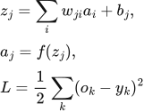 LaTeX:
z_j=\sum_iw_{ji}a_i+b_j,\quad a_j=f(z_j),\quad L=\frac12\sum_k(o_k-y_k)^2Delta means the loss gradient with respect to a neuron's raw score. First calculate output deltas, then hidden deltas using every connected output path.
 LaTeX:
\delta_{o_k}=(o_k-y_k)f'(z_{o_k})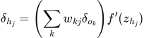 LaTeX:
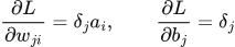
\delta_{h_j}=\left(\sum_kw_{kj}\delta_{o_k}\right)f'(z_{h_j})The gradient of a connection is its receiving delta multiplied by its sending activation. A bias receives the constant 1.
 LaTeX:
\frac{\partial L}{\partial w_{ji}}=\delta_j a_i,\qquad \frac{\partial L}{\partial b_j}=\delta_j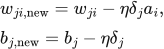 LaTeX:
w_{ji,\mathrm{new}}=w_{ji}-\eta\delta_j a_i,\quad b_{j,\mathrm{new}}=b_j-\eta\delta_jFor sigmoid, use f′ = a(1 − a). For ReLU, use f′ = 1 for a positive raw score and 0 for a negative raw score. Store the old weights until all gradients have been calculated.
Step 1 map the arrows. Each row of W₁ receives all inputs; each row of W₂ receives all hidden outputs. Bias is added once per receiving neuron. All gradients below use the OLD weights from this same forward pass.
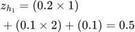
Hidden neuron 1:
 LaTeX:
z_{h_1} = (0.2 \times 1) + (0.1 \times 2) + (0.1) = 0.5 LaTeX:
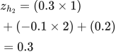
h_{1} = \max(0,0.5) = 0.5Hidden neuron 2:
 LaTeX:
z_{h_2} = (0.3 \times 1) + (-0.1 \times 2) + (0.2) = 0.3 LaTeX:
h_{2} = \max(0,0.3) = 0.3Output neuron 1:
 LaTeX:
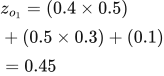
z_{o_1} = (0.4 \times 0.5) + (0.5 \times 0.3) + (0.1) = 0.45 LaTeX:
o_{1} = \max(0,0.45) = 0.45Step 2 loss convention. This worked solution uses half summed squared loss, L = ½Σ(o − y)². Follow the loss specified in the question; where none is supplied, this is an explicit assumption.
Prediction minus target = [-0.55]. Squared errors = [0.3025]. Half-sum squared loss = 0.15125; mean squared error = 0.3025. These are different unless the number of output components makes the scale coincide.
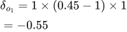
Output delta 1:
 LaTeX:
\delta_{o_1} = 1 \times (0.45-1) \times 1 = -0.55The ReLU derivative is 1 here because this preactivation is positive.
Step 3 output weights. Gradient = receiving delta × sending activation. An output bias gradient equals its delta.
h1 → o1:
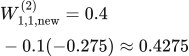
Subtract η × gradient = −0.0275. This weight increases.
The sending value and receiving delta have different roles. All deltas still use the original forward-pass weights.
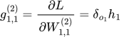
The receiving neuron supplies the delta; the sending neuron supplies its activation.
 LaTeX:
g_{1,1}^{(2)}=\frac{\partial L}{\partial W^{(2)}_{1,1}}=\delta_{o_1}h_1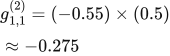 LaTeX:
g_{1,1}^{(2)}=(-0.55)\times(0.5)\approx -0.275Apply the learning rate to this gradient and subtract the result from the old weight.
 LaTeX:
W^{(2)}_{1,1,\mathrm{new}}=0.4-0.1(-0.275)\approx 0.4275h2 → o1:
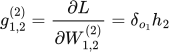
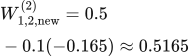
Subtract η × gradient = −0.0165. This weight increases.
The sending value and receiving delta have different roles. All deltas still use the original forward-pass weights.
The receiving neuron supplies the delta; the sending neuron supplies its activation.
 LaTeX:
g_{1,2}^{(2)}=\frac{\partial L}{\partial W^{(2)}_{1,2}}=\delta_{o_1}h_2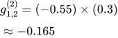 LaTeX:
g_{1,2}^{(2)}=(-0.55)\times(0.3)\approx -0.165Apply the learning rate to this gradient and subtract the result from the old weight.
 LaTeX:
W^{(2)}_{1,2,\mathrm{new}}=0.5-0.1(-0.165)\approx 0.5165Step 4 hidden deltas. A hidden unit can influence EVERY connected output, so add those paths BEFORE multiplying by the hidden activation derivative.
Hidden 1 downstream contribution:
Calculate each outgoing path using the old outgoing weight and that output's delta.
Multiply within each path. Add the resulting contributions at the shared hidden neuron.
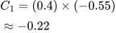
Contribution from output 1.
 LaTeX:
C_1=(0.4)\times(-0.55)\approx -0.22Accumulate the contributions, then apply the hidden activation derivative below.
 LaTeX:
\text{Sum}=C_1\approx -0.22 LaTeX:
\delta_{h_1} = -0.22 \times 1 = -0.22Hidden 2 downstream contribution:
Calculate each outgoing path using the old outgoing weight and that output's delta.
Multiply within each path. Add the resulting contributions at the shared hidden neuron.
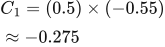
Contribution from output 1.
 LaTeX:
C_1=(0.5)\times(-0.55)\approx -0.275Accumulate the contributions, then apply the hidden activation derivative below.
 LaTeX:
\text{Sum}=C_1\approx -0.275 LaTeX:
\delta_{h_2} = -0.275 \times 1 = -0.275Step 5 input weights. Multiply the hidden delta by the corresponding raw input, not by the hidden output.
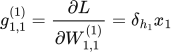
x1 → h1:
Subtract η × gradient = −0.022. This weight increases.
The sending value and receiving delta have different roles. All deltas still use the original forward-pass weights.
The receiving neuron supplies the delta; the sending neuron supplies the input value.
 LaTeX:
g_{1,1}^{(1)}=\frac{\partial L}{\partial W^{(1)}_{1,1}}=\delta_{h_1}x_1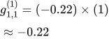 LaTeX:
g_{1,1}^{(1)}=(-0.22)\times(1)\approx -0.22Apply the learning rate to this gradient and subtract the result from the old weight.
 LaTeX:
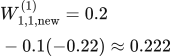
W^{(1)}_{1,1,\mathrm{new}}=0.2-0.1(-0.22)\approx 0.222x2 → h1:
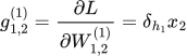
Subtract η × gradient = −0.044. This weight increases.
The sending value and receiving delta have different roles. All deltas still use the original forward-pass weights.
The receiving neuron supplies the delta; the sending neuron supplies the input value.
 LaTeX:
g_{1,2}^{(1)}=\frac{\partial L}{\partial W^{(1)}_{1,2}}=\delta_{h_1}x_2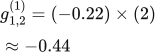 LaTeX:
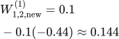
g_{1,2}^{(1)}=(-0.22)\times(2)\approx -0.44Apply the learning rate to this gradient and subtract the result from the old weight.
 LaTeX:
W^{(1)}_{1,2,\mathrm{new}}=0.1-0.1(-0.44)\approx 0.144x1 → h2:
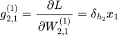
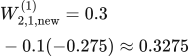
Subtract η × gradient = −0.0275. This weight increases.
The sending value and receiving delta have different roles. All deltas still use the original forward-pass weights.
The receiving neuron supplies the delta; the sending neuron supplies the input value.
 LaTeX:
g_{2,1}^{(1)}=\frac{\partial L}{\partial W^{(1)}_{2,1}}=\delta_{h_2}x_1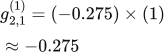 LaTeX:
g_{2,1}^{(1)}=(-0.275)\times(1)\approx -0.275Apply the learning rate to this gradient and subtract the result from the old weight.
 LaTeX:
W^{(1)}_{2,1,\mathrm{new}}=0.3-0.1(-0.275)\approx 0.3275x2 → h2:
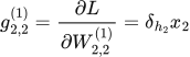
Subtract η × gradient = −0.055. This weight increases.
The sending value and receiving delta have different roles. All deltas still use the original forward-pass weights.
The receiving neuron supplies the delta; the sending neuron supplies the input value.
 LaTeX:
g_{2,2}^{(1)}=\frac{\partial L}{\partial W^{(1)}_{2,2}}=\delta_{h_2}x_2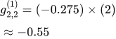 LaTeX:
g_{2,2}^{(1)}=(-0.275)\times(2)\approx -0.55Apply the learning rate to this gradient and subtract the result from the old weight.
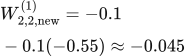 LaTeX:
W^{(1)}_{2,2,\mathrm{new}}=-0.1-0.1(-0.55)\approx -0.045Step 6 bias updates. A bias receives a constant input 1, so its gradient equals the corresponding delta. Use the same old forward pass and learning rate as the weight updates.
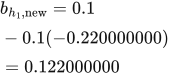 LaTeX:
b_{h_1,\mathrm{new}}=0.1-0.1(-0.220000000)=0.122000000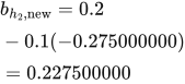 LaTeX:
b_{h_2,\mathrm{new}}=0.2-0.1(-0.275000000)=0.227500000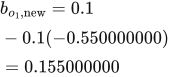 LaTeX:
b_{o_1,\mathrm{new}}=0.1-0.1(-0.550000000)=0.155000000These are independent per-neuron biases. If the question fixes biases, keep them fixed. If it specifies a single tied bias, add all deltas sharing that bias before updating it.
Drill 12 Two output sigmoid backpropagation
Question
Question. Input x = [0.2, 0.4]. Each row below lists the incoming weights of one receiving neuron. W₁ is shown below; b₁ = [0.1, 0.1]; W₂ is shown below; b₂ = [0, 0.1]. Hidden and output activations are sigmoid. Target y = [1, 0]. Learning rate η = 0.2. Use half summed squared loss and update all parameters.
Answer — step by step
Given
Input x = [0.2, 0.4].
W₁ is printed with the question.
b₁ = [0.1, 0.1].
W₂ is printed with the question.
b₂ = [0, 0.1].
Hidden and output activations are sigmoid.
Target y = [1, 0].
Learning rate η = 0.2.
Use half summed squared loss and update all parameters.
To find
Find all preactivations, hidden activations and final outputs. Calculate the half summed squared loss and its output derivatives. Find the sigmoid output and, if requested, its derivative. Find the requested deltas and parameter gradients, then update the specified parameters.
Formula — which one and why
Forward propagation. Evaluate one layer completely before supplying its activated outputs to the next layer. Each layer has its own weights and biases.
x = input vector; h = hidden outputs; W₁,b₁ = hidden parameters; W₂,b₂ = output parameters; f₁,f₂ = the stated activations.
LaTeX: z_h=W_1x+b_1LaTeX: h=f_1(z_h)LaTeX: z_o=W_2h+b_2LaTeX: o=f_2(z_o)Yaad rakhne ka cue: Pehli layer ka activated output hi agli layer ka input hai.
Half summed squared loss. This loss convention takes one-half of the sum of squared prediction errors. Use it when the question specifies it, or explicitly state it as an assumption when the paper omits the loss. Differentiating cancels the factor one-half against the square derivative.
oⱼ = output j; yⱼ = target j; L = half summed squared loss under the stated or explicitly assumed convention.
LaTeX: L=\frac12\sum_j(o_j-y_j)^2LaTeX: \frac{\partial L}{\partial o_j}=o_j-y_jYaad rakhne ka cue: Half aur square ka 2 cancel: output derivative = prediction − target.
Sigmoid and its slope. Use sigmoid when the neuron is specified to squash its preactivation into (0,1). Once its output is known, its derivative needs only output × (1−output).
z = preactivation; p = sigmoid output; e is the exponential base, not a prediction error in this formula.
 LaTeX:
p=\frac{1}{1+e^{-z}}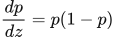 LaTeX:
\frac{dp}{dz}=p(1-p)Yaad rakhne ka cue: Sigmoid output p; uska slope p × (1−p).
Backpropagation. The loss tells us how each output must change. Multiply by that neuron’s activation slope to obtain its delta. A weight gradient is receiving delta × sending value. Hidden deltas must include every outgoing path.
δ (delta) = derivative of loss with respect to a neuron’s preactivation; f′ = activation derivative; aᵢ = sending activation; Wⱼᵢ = connection weight. Use the exact loss scaling in the question.
LaTeX: \delta_{o_j}=\frac{\partial L}{\partial o_j}f_o\prime(z_{o_j})LaTeX: \delta_{h_i}=f_h\prime(z_{h_i})\sum_jW_{ji}^{(2)}\delta_{o_j}LaTeX: \frac{\partial L}{\partial W_{ji}}=\delta_ja_iLaTeX: \frac{\partial L}{\partial b_j}=\delta_jLaTeX: W_{ji,\mathrm{new}}=W_{ji}-\eta\frac{\partial L}{\partial W_{ji}}Yaad rakhne ka cue: Receiving delta × sending value = us connection ka gradient.
Solution — step by step
Formulas used before substituting numbers
For every receiving neuron, z is its weighted sum and a is its activated output. The half squared loss sums the errors from all output neurons.
LaTeX: z_j=\sum_iw_{ji}a_i+b_j,\quad a_j=f(z_j),\quad L=\frac12\sum_k(o_k-y_k)^2Delta means the loss gradient with respect to a neuron's raw score. First calculate output deltas, then hidden deltas using every connected output path.
LaTeX: \delta_{o_k}=(o_k-y_k)f'(z_{o_k})LaTeX: \delta_{h_j}=\left(\sum_kw_{kj}\delta_{o_k}\right)f'(z_{h_j})The gradient of a connection is its receiving delta multiplied by its sending activation. A bias receives the constant 1.
LaTeX: \frac{\partial L}{\partial w_{ji}}=\delta_j a_i,\qquad \frac{\partial L}{\partial b_j}=\delta_jLaTeX: w_{ji,\mathrm{new}}=w_{ji}-\eta\delta_j a_i,\quad b_{j,\mathrm{new}}=b_j-\eta\delta_jFor sigmoid, use f′ = a(1 − a). For ReLU, use f′ = 1 for a positive raw score and 0 for a negative raw score. Store the old weights until all gradients have been calculated.
Step 1 map the arrows. Each row of W₁ receives all inputs; each row of W₂ receives all hidden outputs. Bias is added once per receiving neuron. All gradients below use the OLD weights from this same forward pass.
Hidden neuron 1:
 LaTeX:
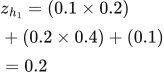
z_{h_1} = (0.1 \times 0.2) + (0.2 \times 0.4) + (0.1) = 0.2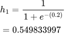 LaTeX:
h_{1}=\frac{1}{1+e^{-(0.2)}}=0.549833997Hidden neuron 2:
 LaTeX:
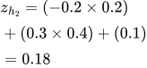
z_{h_2} = (-0.2 \times 0.2) + (0.3 \times 0.4) + (0.1) = 0.18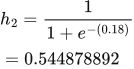 LaTeX:
h_{2}=\frac{1}{1+e^{-(0.18)}}=0.544878892Output neuron 1:
 LaTeX:
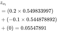
z_{o_1} = (0.2 \times 0.549833997) + (-0.1 \times 0.544878892) + (0) = 0.05547891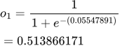 LaTeX:
o_{1}=\frac{1}{1+e^{-(0.05547891)}}=0.513866171Output neuron 2:
 LaTeX:
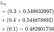
z_{o_2} = (0.3 \times 0.549833997) + (0.4 \times 0.544878892) + (0.1) = 0.482901756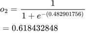 LaTeX:
o_{2}=\frac{1}{1+e^{-(0.482901756)}}=0.618432848Step 2 loss convention. This worked solution uses half summed squared loss, L = ½Σ(o − y)². Follow the loss specified in the question; where none is supplied, this is an explicit assumption.
Prediction minus target = [-0.486133829, 0.618432848]. Squared errors = [0.2363261, 0.382459187]. Half-sum squared loss = 0.309392643; mean squared error = 0.309392643. These are different unless the number of output components makes the scale coincide.
Output delta 1:
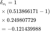 LaTeX:
\delta_{o_1} = 1 \times (0.513866171-1) \times 0.249807729 = -0.121439988The derivative is o(1−o).
Output delta 2:
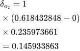 LaTeX:
\delta_{o_2} = 1 \times (0.618432848-0) \times 0.235973661 = 0.145933863The derivative is o(1−o).
Step 3 output weights. Gradient = receiving delta × sending activation. An output bias gradient equals its delta.
h1 → o1:
Subtract η × gradient = −0.013354367. This weight increases.
The sending value and receiving delta have different roles. All deltas still use the original forward-pass weights.
The receiving neuron supplies the delta; the sending neuron supplies its activation.
LaTeX: g_{1,1}^{(2)}=\frac{\partial L}{\partial W^{(2)}_{1,1}}=\delta_{o_1}h_1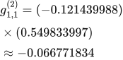 LaTeX:
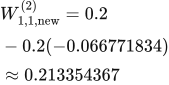
g_{1,1}^{(2)}=(-0.121439988)\times(0.549833997)\approx -0.066771834Apply the learning rate to this gradient and subtract the result from the old weight.
 LaTeX:
W^{(2)}_{1,1,\mathrm{new}}=0.2-0.2(-0.066771834)\approx 0.213354367h2 → o1:
Subtract η × gradient = −0.013234017. This weight increases.
The sending value and receiving delta have different roles. All deltas still use the original forward-pass weights.
The receiving neuron supplies the delta; the sending neuron supplies its activation.
LaTeX: g_{1,2}^{(2)}=\frac{\partial L}{\partial W^{(2)}_{1,2}}=\delta_{o_1}h_2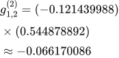 LaTeX:
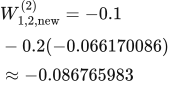
g_{1,2}^{(2)}=(-0.121439988)\times(0.544878892)\approx -0.066170086Apply the learning rate to this gradient and subtract the result from the old weight.
 LaTeX:
W^{(2)}_{1,2,\mathrm{new}}=-0.1-0.2(-0.066170086)\approx -0.086765983h1 → o2:
Subtract η × gradient = 0.01604788. This weight decreases.
The sending value and receiving delta have different roles. All deltas still use the original forward-pass weights.
The receiving neuron supplies the delta; the sending neuron supplies its activation.
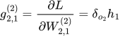 LaTeX:
g_{2,1}^{(2)}=\frac{\partial L}{\partial W^{(2)}_{2,1}}=\delta_{o_2}h_1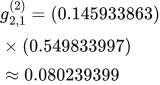 LaTeX:
g_{2,1}^{(2)}=(0.145933863)\times(0.549833997)\approx 0.080239399Apply the learning rate to this gradient and subtract the result from the old weight.
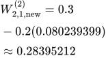 LaTeX:
W^{(2)}_{2,1,\mathrm{new}}=0.3-0.2(0.080239399)\approx 0.28395212h2 → o2:
Subtract η × gradient = 0.015903256. This weight decreases.
The sending value and receiving delta have different roles. All deltas still use the original forward-pass weights.
The receiving neuron supplies the delta; the sending neuron supplies its activation.
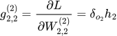 LaTeX:
g_{2,2}^{(2)}=\frac{\partial L}{\partial W^{(2)}_{2,2}}=\delta_{o_2}h_2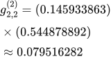 LaTeX:
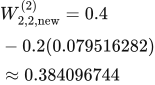
g_{2,2}^{(2)}=(0.145933863)\times(0.544878892)\approx 0.079516282Apply the learning rate to this gradient and subtract the result from the old weight.
 LaTeX:
W^{(2)}_{2,2,\mathrm{new}}=0.4-0.2(0.079516282)\approx 0.384096744Step 4 hidden deltas. A hidden unit can influence EVERY connected output, so add those paths BEFORE multiplying by the hidden activation derivative.
Hidden 1 downstream contribution:
Calculate each outgoing path using the old outgoing weight and that output's delta.
Multiply within each path. Add the resulting contributions at the shared hidden neuron.
Contribution from output 1.
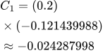 LaTeX:
C_1=(0.2)\times(-0.121439988)\approx -0.024287998Contribution from output 2.
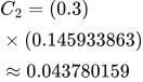 LaTeX:
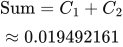
C_2=(0.3)\times(0.145933863)\approx 0.043780159Accumulate the contributions, then apply the hidden activation derivative below.
 LaTeX:
\text{Sum}=C_1+C_2\approx 0.019492161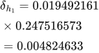 LaTeX:
\delta_{h_1} = 0.019492161 \times 0.247516573 = 0.004824633Hidden 2 downstream contribution:
Calculate each outgoing path using the old outgoing weight and that output's delta.
Multiply within each path. Add the resulting contributions at the shared hidden neuron.
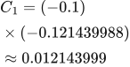
Contribution from output 1.
 LaTeX:
C_1=(-0.1)\times(-0.121439988)\approx 0.012143999Contribution from output 2.
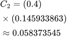 LaTeX:
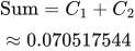
C_2=(0.4)\times(0.145933863)\approx 0.058373545Accumulate the contributions, then apply the hidden activation derivative below.
 LaTeX:
\text{Sum}=C_1+C_2\approx 0.070517544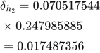 LaTeX:
\delta_{h_2} = 0.070517544 \times 0.247985885 = 0.017487356Step 5 input weights. Multiply the hidden delta by the corresponding raw input, not by the hidden output.
x1 → h1:
Subtract η × gradient = 0.000192985. This weight decreases.
The sending value and receiving delta have different roles. All deltas still use the original forward-pass weights.
The receiving neuron supplies the delta; the sending neuron supplies the input value.
LaTeX: g_{1,1}^{(1)}=\frac{\partial L}{\partial W^{(1)}_{1,1}}=\delta_{h_1}x_1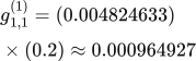 LaTeX:
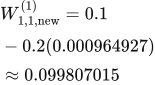
g_{1,1}^{(1)}=(0.004824633)\times(0.2)\approx 0.000964927Apply the learning rate to this gradient and subtract the result from the old weight.
 LaTeX:
W^{(1)}_{1,1,\mathrm{new}}=0.1-0.2(0.000964927)\approx 0.099807015x2 → h1:
Subtract η × gradient = 0.000385971. This weight decreases.
The sending value and receiving delta have different roles. All deltas still use the original forward-pass weights.
The receiving neuron supplies the delta; the sending neuron supplies the input value.
LaTeX: g_{1,2}^{(1)}=\frac{\partial L}{\partial W^{(1)}_{1,2}}=\delta_{h_1}x_2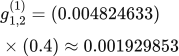 LaTeX:
g_{1,2}^{(1)}=(0.004824633)\times(0.4)\approx 0.001929853Apply the learning rate to this gradient and subtract the result from the old weight.
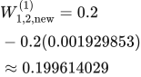 LaTeX:
W^{(1)}_{1,2,\mathrm{new}}=0.2-0.2(0.001929853)\approx 0.199614029x1 → h2:
Subtract η × gradient = 0.000699494. This weight decreases.
The sending value and receiving delta have different roles. All deltas still use the original forward-pass weights.
The receiving neuron supplies the delta; the sending neuron supplies the input value.
LaTeX: g_{2,1}^{(1)}=\frac{\partial L}{\partial W^{(1)}_{2,1}}=\delta_{h_2}x_1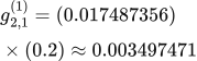 LaTeX:
g_{2,1}^{(1)}=(0.017487356)\times(0.2)\approx 0.003497471Apply the learning rate to this gradient and subtract the result from the old weight.
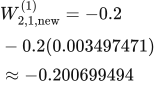 LaTeX:
W^{(1)}_{2,1,\mathrm{new}}=-0.2-0.2(0.003497471)\approx -0.200699494x2 → h2:
Subtract η × gradient = 0.001398988. This weight decreases.
The sending value and receiving delta have different roles. All deltas still use the original forward-pass weights.
The receiving neuron supplies the delta; the sending neuron supplies the input value.
LaTeX: g_{2,2}^{(1)}=\frac{\partial L}{\partial W^{(1)}_{2,2}}=\delta_{h_2}x_2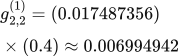 LaTeX:
g_{2,2}^{(1)}=(0.017487356)\times(0.4)\approx 0.006994942Apply the learning rate to this gradient and subtract the result from the old weight.
 LaTeX:
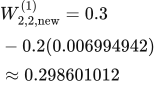
W^{(1)}_{2,2,\mathrm{new}}=0.3-0.2(0.006994942)\approx 0.298601012Step 6 bias updates. A bias receives a constant input 1, so its gradient equals the corresponding delta. Use the same old forward pass and learning rate as the weight updates.
 LaTeX:
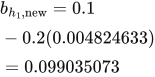
b_{h_1,\mathrm{new}}=0.1-0.2(0.004824633)=0.099035073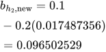 LaTeX:
b_{h_2,\mathrm{new}}=0.1-0.2(0.017487356)=0.096502529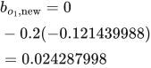 LaTeX:
b_{o_1,\mathrm{new}}=0-0.2(-0.121439988)=0.024287998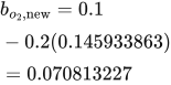 LaTeX:
b_{o_2,\mathrm{new}}=0.1-0.2(0.145933863)=0.070813227These are independent per-neuron biases. If the question fixes biases, keep them fixed. If it specifies a single tied bias, add all deltas sharing that bias before updating it.
Drill 13 A negative ReLU blocks this path
Question
Question. x = 2, w1 = −0.4, b1 = 0.1, w2 = 0.5, b2 = 0.2; hidden ReLU, linear output, y = 1, half squared loss. Find dw 1 and dw 2.
Answer — step by step
Given
x = 2; w₁ = −0.4; b₁ = 0.1; w₂ = 0.5; b₂ = 0.2.
Hidden activation: ReLU; output activation: linear.
Target y = 1; loss: half squared error.
To find
Find the gradients of w₁ and w₂ and explain any zero gradients.
Formula — which one and why
Forward propagation. Evaluate one layer completely before supplying its activated outputs to the next layer. Each layer has its own weights and biases.
x = input vector; h = hidden outputs; W₁,b₁ = hidden parameters; W₂,b₂ = output parameters; f₁,f₂ = the stated activations.
LaTeX: z_h=W_1x+b_1LaTeX: h=f_1(z_h)LaTeX: z_o=W_2h+b_2LaTeX: o=f_2(z_o)Yaad rakhne ka cue: Pehli layer ka activated output hi agli layer ka input hai.
Half summed squared loss. This loss convention takes one-half of the sum of squared prediction errors. Use it when the question specifies it, or explicitly state it as an assumption when the paper omits the loss. Differentiating cancels the factor one-half against the square derivative.
oⱼ = output j; yⱼ = target j; L = half summed squared loss under the stated or explicitly assumed convention.
LaTeX: L=\frac12\sum_j(o_j-y_j)^2LaTeX: \frac{\partial L}{\partial o_j}=o_j-y_jYaad rakhne ka cue: Half aur square ka 2 cancel: output derivative = prediction − target.
Backpropagation. The loss tells us how each output must change. Multiply by that neuron’s activation slope to obtain its delta. A weight gradient is receiving delta × sending value. Hidden deltas must include every outgoing path.
δ (delta) = derivative of loss with respect to a neuron’s preactivation; f′ = activation derivative; aᵢ = sending activation; Wⱼᵢ = connection weight. Use the exact loss scaling in the question.
LaTeX: \delta_{o_j}=\frac{\partial L}{\partial o_j}f_o\prime(z_{o_j})LaTeX: \delta_{h_i}=f_h\prime(z_{h_i})\sum_jW_{ji}^{(2)}\delta_{o_j}LaTeX: \frac{\partial L}{\partial W_{ji}}=\delta_ja_iLaTeX: \frac{\partial L}{\partial b_j}=\delta_jLaTeX: W_{ji,\mathrm{new}}=W_{ji}-\eta\frac{\partial L}{\partial W_{ji}}Yaad rakhne ka cue: Receiving delta × sending value = us connection ka gradient.
Solution — step by step
Formulas used
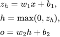
The hidden neuron uses ReLU, but the output is linear. “Linear output” means its weighted sum is already its output.
 LaTeX:
z_h=w_1x+b_1,\quad h=\max(0,z_h),\quad o=w_2h+b_2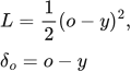 LaTeX:
L=\frac12(o-y)^2,\quad \delta_o=o-y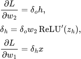 LaTeX:
\frac{\partial L}{\partial w_2}=\delta_o h,\quad \delta_h=\delta_o w_2\operatorname{ReLU}'(z_h),\quad \frac{\partial L}{\partial w_1}=\delta_h xStep 1: hidden weighted sum and activation
 LaTeX:
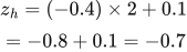
z_h=(-0.4)\times2+0.1=-0.8+0.1=-0.7 LaTeX:
h=\max(0,-0.7)=0Because the raw hidden score is negative, ReLU's derivative at this point is 0.
Step 2: output prediction and output delta
 LaTeX:
o=0.5\times0+0.2=0.2 LaTeX:
\delta_o=0.2-1=-0.8Step 3: output weight gradient
 LaTeX:
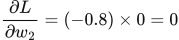
\frac{\partial L}{\partial w_2}=(-0.8)\times0=0This is zero because the input to that connection, h, is zero.
Step 4: hidden delta and input weight gradient
 LaTeX:
\delta_h=(-0.8)\times0.5\times0=0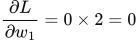 LaTeX:
\frac{\partial L}{\partial w_1}=0\times2=0Final answer: both requested weight gradients are zero. The output bias gradient equals −0.8, so a zero weight gradient does not mean every parameter's gradient is zero.