Deep Learning · MT2 · formulas
Batch and mini-batch gradient
A batch is a group of training examples used together for one update. An epoch is one pass through the dataset. Averaging gradients and counting updates are different questions, so both receive complete worked examples below.
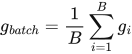 LaTeX:
g_{batch}=\frac1B\sum_{i=1}^{B}g_i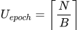 LaTeX:
U_{epoch}=\left\lceil\frac NB\right\rceilModel answer: batch, stochastic and mini-batch training
Question
Question. Differentiate batch gradient descent, stochastic gradient descent and mini-batch gradient descent. Explain an epoch, a batch and an iteration.
Answer — step by step
All three methods update model parameters using gradients. Their difference is the number of training examples used to estimate the gradient for one update.
A batch is the group of examples used together for an update. An iteration, in this context, is one optimizer update. An epoch is one complete pass through the chosen training dataset. One epoch usually contains several iterations.
| Basis | Batch GD | Stochastic GD | Mini-batch GD |
|---|---|---|---|
| Examples in one gradient | Entire training dataset | One example | A smaller group of B examples |
| Updates per epoch | One | N | Ceiling of N/B if the remainder is retained |
| Gradient behavior | Full-data gradient | Noisy sample gradient | Intermediate averaging |
| Practical implication | Updates can be expensive on large datasets | Many small, sequential updates | Common compromise for vectorized computation |
Example to distinguish the three counts
With 105 examples and batch size 20, five batches use 100 examples and a sixth uses the remaining 5. Therefore one epoch has 6 mini-batch updates. Three epochs give 18 updates. It would be 5 updates per epoch only if the problem explicitly discarded the incomplete batch.
The basic parameter update is unchanged:
 LaTeX:
\theta_{\mathrm{new}}=\theta_{\mathrm{old}}-\eta gFor batch or mini-batch training, g normally represents the gradient of the stated aggregate loss over that group. For sequential SGD, update after each example and use the new parameter for the next example. Consequently, one SGD epoch need not equal one batch update even when both use the same examples.
A tiny dataset shows why the methods differ
Question. Train ŷ = wx on samples (1,2) and (2,4), starting at w = 1, with η = 0.1 and mean half squared loss. Compare one batch update with one SGD epoch in the listed order.
Given
Model ŷ = wx; initial w = 1; η = 0.1.
Samples in order: (1,2), (2,4).
Mean half squared loss for the batch.
To find
Compare one batch update with a sequential SGD epoch.
Formula — which one and why
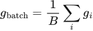
Batch mean versus sequential SGD. A batch update averages gradients evaluated at the same old parameter. Sequential SGD updates after each sample, so later samples use the changed parameter.
B = number of examples in the batch; gᵢ = sample gradient; η = learning rate. For the linear half squared objective, sample gradient is (wx−y)x.
 LaTeX:
g_{\mathrm{batch}}=\frac1B\sum_i g_i LaTeX:
g_i=(wx_i-y_i)x_i LaTeX:
w_{\mathrm{new}}=w-\eta gYaad rakhne ka cue: Batch: same old weight par average; SGD: har sample ke baad weight change.
Solution — step by step
One batch update
Step 1: predict sample 1 with the original weight.
 LaTeX:
\hat y_1=1(1)=1Step 2: calculate its error.
 LaTeX:
e_1=1-2=-1Step 3: multiply its error by its input.
 LaTeX:
g_1=(-1)(1)=-1Step 4: predict sample 2 with the same original weight.
 LaTeX:
\hat y_2=1(2)=2Step 5: calculate its error.
 LaTeX:
e_2=2-4=-2Step 6: multiply its error by its input.
 LaTeX:
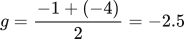
g_2=(-2)(2)=-4Step 7: average the two gradients.
 LaTeX:
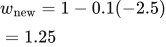
g=\frac{-1+(-4)}2=-2.5Step 8: update once.
 LaTeX:
w_{\mathrm{new}}=1-0.1(-2.5)=1.25One sequential SGD epoch
Step 1: use the first sample gradient.
 LaTeX:
g_1=-1Step 2: update after the first sample.
 LaTeX:
w_1=1-0.1(-1)=1.1Step 3: predict sample 2 using the changed weight.
 LaTeX:
\hat y_2=1.1(2)=2.2Step 4: find sample 2 error.
 LaTeX:
e_2=2.2-4=-1.8Step 5: find the new sample 2 gradient.
 LaTeX:
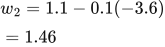
g_2=(-1.8)(2)=-3.6Step 6: update after sample 2.
 LaTeX:
w_2=1.1-0.1(-3.6)=1.46Final answer: batch weight = 1.25; sequential SGD weight = 1.46. SGD changes the weight between samples.
Larger mini-batches use more memory and often make better use of parallel hardware. Smaller batches provide noisier gradient estimates and more updates per epoch. Wall-clock speed and generalization depend on the implementation and problem, so “SGD always converges fastest” is not a safe claim.
Drill 14 Batch and sequential SGD
Question
Question. ŷ = wx, start w = 0, η = 0.1, data(1,1), (2,2). Use mean half squared loss for a batch. Compare one batch update with one sequential SGD epoch.
Answer — step by step
Given
Model ŷ = wx; initial w = 0; η = 0.1.
Samples in order: (x,y) = (1,1), then (2,2).
Batch objective: mean half squared loss.
To find
Compare the weight after one batch update and one sequential SGD epoch.
Formula — which one and why
Batch mean versus sequential SGD. A batch update averages gradients evaluated at the same old parameter. Sequential SGD updates after each sample, so later samples use the changed parameter.
B = number of examples in the batch; gᵢ = sample gradient; η = learning rate. For the linear half squared objective, sample gradient is (wx−y)x.
LaTeX: g_{\mathrm{batch}}=\frac1B\sum_i g_iLaTeX: g_i=(wx_i-y_i)x_iLaTeX: w_{\mathrm{new}}=w-\eta gYaad rakhne ka cue: Batch: same old weight par average; SGD: har sample ke baad weight change.
Solution — step by step
Meaning and formulas
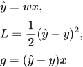
For one sample, x is the input, y is the target, and w is the weight. Batch GD averages gradients evaluated at the same old weight. Sequential SGD updates after each sample and uses that new weight for the next sample.
 LaTeX:
\hat y=wx,\quad L=\frac12(\hat y-y)^2,\quad g=(\hat y-y)x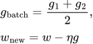 LaTeX:
g_{\mathrm{batch}}=\frac{g_1+g_2}{2},\qquad w_{\mathrm{new}}=w-\eta gStep 1: Part A: one batch update from w = 0.
For sample (1,1), prediction = 0 × 1 = 0, so:
 LaTeX:
g_1=(0-1)\times1=-1For sample (2,2), keep the same weight 0. Prediction = 0 × 2 = 0, so:
 LaTeX:
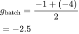
g_2=(0-2)\times2=-4Average these two gradients, then update once.
 LaTeX:
g_{\mathrm{batch}}=\frac{-1+(-4)}2=-2.5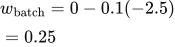 LaTeX:
w_{\mathrm{batch}}=0-0.1(-2.5)=0.25Step 2: Part B: one SGD epoch, restarting at w = 0.
The first sample has gradient −1, just as above.
 LaTeX:
w_1=0-0.1(-1)=0.1For the second sample use this new weight, so prediction is:
 LaTeX:
\hat y_2=0.1\times2=0.2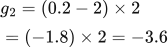 LaTeX:
g_2=(0.2-2)\times2=(-1.8)\times2=-3.6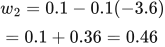 LaTeX:
w_2=0.1-0.1(-3.6)=0.1+0.36=0.46Final answer: batch result 0.25; sequential SGD result 0.46. The difference comes from the timing of the updates.
Drill 15 Incomplete mini batch
Question
Question. N = 103, B = 20, epochs = 3. Count updates for batch GD, SGD, mini-batch keeping the remainder, and mini-batch dropping it.
Answer — step by step
Given
N = 103 samples; B = 20 samples per mini-batch.
E = 3 epochs.
Compare both remainder policies: keep or drop the final 3 examples.
To find
Find total updates for full-batch GD, SGD, and both mini-batch policies.
Formula — which one and why
Number of updates. An update occurs after one processed batch. Full-batch GD uses one batch per epoch; SGD uses one sample per batch. Mini-batches need a stated remainder policy.
N = dataset size; B = batch size; E = number of epochs. Ceiling rounds upward to include a smaller final batch; floor drops it.
 LaTeX:
U_{\mathrm{batch}}=E LaTeX:
U_{\mathrm{SGD}}=EN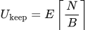 LaTeX:
U_{\mathrm{keep}}=E\left\lceil\frac NB\right\rceil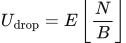 LaTeX:
U_{\mathrm{drop}}=E\left\lfloor\frac NB\right\rfloorYaad rakhne ka cue: Kitne batches process hue, utne updates hue.
Solution — step by step
Meaning and formulas
An epoch means one pass through the dataset. An update happens once per batch used. N is the number of samples, B is the chosen batch size, and E is the number of epochs.
 LaTeX:
U_{\mathrm{batch}}=E,\qquad U_{\mathrm{SGD}}=NE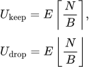 LaTeX:
U_{\mathrm{keep}}=E\left\lceil\frac NB\right\rceil,\qquad U_{\mathrm{drop}}=E\left\lfloor\frac NB\right\rfloorCeiling rounds up to the next integer; floor rounds down. The final incomplete batch needs an update only if it is retained.
Step 1: batch GD
All 103 samples form one batch per epoch.
 LaTeX:
U_{\mathrm{batch}}=3\times1=3Step 2: SGD
Each sample gets its own update.
 LaTeX:
U_{\mathrm{SGD}}=103\times3=309Step 3: mini-batches with the remainder
 LaTeX:
103=5\times20+3The batch sizes are 20, 20, 20, 20, 20 and 3. Six batches per epoch give:
 LaTeX:
U_{\mathrm{keep}}=6\times3=18Step 4: mini-batches without the remainder
Only the five complete batches are used each epoch.
 LaTeX:
U_{\mathrm{drop}}=5\times3=15Final answer: 3, 309, 18 and 15 updates respectively.