Deep Learning · MT2 · formulas
RMSProp
RMSProp remembers a weighted average of squared gradients. With decay 0.9, keep 90% of the old stored value and add 10% of the new squared gradient. Calculate this new stored value before taking its square root and updating the parameter.
 LaTeX:
s_t=\rho s_{t-1}+(1-\rho)g_t^2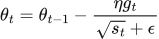 LaTeX:
\theta_t=\theta_{t-1}-\frac{\eta g_t}{\sqrt{s_t}+\epsilon}A moving average remembers the recent past
Definition. An exponentially weighted moving average (EWMA) is a recursively updated estimate in which older observations receive exponentially decreasing weights. Optimizers use it to summarize recent gradients or squared gradients.
 LaTeX:
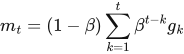
m_t=\beta m_{t-1}+(1-\beta)g_t,\qquad0\le\beta<1For m₀ = 0, expanding the recurrence gives:
 LaTeX:
m_t=(1-\beta)\sum_{k=1}^{t}\beta^{t-k}g_kThe most recent gradient has coefficient 1 − β; a gradient k steps older is discounted by an additional factor βᵏ. Larger β smooths more strongly but responds more slowly to a change in direction. The heuristic averaging horizon is approximately 1/(1 − β); it is not a hard cutoff in the stored history.
Signed gradients versus squared gradients
An average of g contains directional information: positive and negative contributions can cancel. An average of g² estimates the scale through an uncentered second moment and cannot become negative when initialized nonnegatively. Adam tracks both quantities. RMSProp tracks a squared-gradient average in its basic form.
Question. Let β = 0.9, m₀ = 0 and gradients g₁ = 2, g₂ = −1. Find m₁ and m₂.
Given
β = 0.9; initial m₀ = 0.
Gradients in order: g₁ = 2, g₂ = −1.
To find
Find m₁ and m₂, preserving the sign of each gradient.
Formula — which one and why
Exponential moving average. Keep the specified fraction of the old state and add the complementary fraction of the new gradient. This tracks signed direction, so negative gradients can reduce the state.
β (beta) = retained fraction; m = stored average; g = current gradient. m₀ is the initial state.
 LaTeX:
m_t=\beta m_{t-1}+(1-\beta)g_tYaad rakhne ka cue: Beta purani memory rakhta hai; 1−beta naya gradient leta hai.
Solution — step by step
Step 1: find the recent-gradient coefficient.
 LaTeX:
1-0.9=0.1Step 2: retain the old memory for step 1.
 LaTeX:
0.9(0)=0Step 3: weight the first gradient.
 LaTeX:
0.1(2)=0.2Step 4: add to obtain the first memory.
 LaTeX:
m_1=0+0.2=0.2Step 5: retain the first memory for step 2.
 LaTeX:
0.9(0.2)=0.18Step 6: weight the second gradient.
 LaTeX:
0.1(-1)=-0.1Step 7: add to obtain the second memory.
 LaTeX:
m_2=0.18+(-0.1)=0.08Final answer: m₁ = 0.2; m₂ = 0.08.
The second average remains positive although the latest gradient is negative because the previous positive contribution still has weight. If the recurrence is applied to the squared gradients instead, the second state is 0.9(0.4) + 0.1(1) = 0.46. These states have different meanings and are not interchangeable.
RMSProp remembers recent squared gradients
Definition. RMSProp is an adaptive optimizer that normalizes the current gradient by the root of an exponentially weighted moving average of squared gradients. Its decaying history addresses AdaGrad's permanently growing accumulator.
Recurrence and interpretation
Using decay β and zero initial state:
 LaTeX:
s_t=\beta s_{t-1}+(1-\beta)g_t^2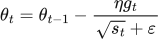 LaTeX:
\theta_t=\theta_{t-1}-\frac{\eta g_t}{\sqrt{s_t}+\varepsilon}β is the fraction of the previous squared-gradient average retained, not a signed velocity. Some papers use ρ for this same decay. The square is applied to the gradient before averaging; the square root is applied to the resulting average in the update.
If recent squared gradients are smaller than the old average, s can decrease. Thus older large gradients do not remain in the denominator with their original weight forever.
Complete numerical: two iterations
Question. θ₀ = 1, s₀ = 0, η = 0.1, β = 0.9; supplied gradients are 2 then 1. Perform two RMSProp updates, with ε = 0 for this hand calculation.
Given
θ₀ = 1; initial state(s) = 0; η = 0.1.
Supplied gradients g₁ = 2, g₂ = 1.
ε = 0 for this hand calculation.
β = 0.9.
To find
Calculate all required states and the parameter after each of two updates.
Formula — which one and why
RMSProp. Use a decaying average of squared gradients, then scale the current gradient by its square root. Old contributions gradually lose influence.
s = squared-gradient average; ρ (rho), sometimes written β, = retained fraction; g = current gradient; η = learning rate; ε = denominator stabilizer.
LaTeX: s_t=\rho s_{t-1}+(1-\rho)g_t^2LaTeX: \theta_t=\theta_{t-1}-\frac{\eta g_t}{\sqrt{s_t}+\epsilon}Yaad rakhne ka cue: Saare purane squares nahi—unki fading average.
Solution — step by step
Iteration 1 — step 1: calculate the squared-gradient average.
 LaTeX:
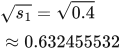
s_1=0.9(0)+0.1(2^2)=0.4Step 2: calculate the denominator and signed correction.
 LaTeX:
\sqrt{s_1}=\sqrt{0.4}\approx0.632455532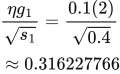 LaTeX:
\frac{\eta g_1}{\sqrt{s_1}}=\frac{0.1(2)}{\sqrt{0.4}}\approx0.316227766Step 3: update the parameter.
 LaTeX:
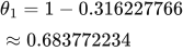
\theta_1=1-0.316227766\approx0.683772234Iteration 2 — step 1: use s₁, not the original zero state.
 LaTeX:
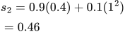
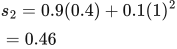
s_2=0.9(0.4)+0.1(1^2)=0.46Step 2: calculate the denominator and signed correction.
 LaTeX:
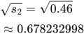
\sqrt{s_2}=\sqrt{0.46}\approx0.678232998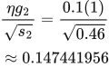 LaTeX:
\frac{\eta g_2}{\sqrt{s_2}}=\frac{0.1(1)}{\sqrt{0.46}}\approx0.147441956Step 3: update from θ₁, retaining calculator precision.
 LaTeX:
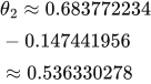
\theta_2\approx0.683772234-0.147441956\approx0.536330278Final answer: θ₁ ≈ 0.683772 and θ₂ ≈ 0.536330; s₁ = 0.4 and s₂ = 0.46.
Comparison with AdaGrad and Adam
AdaGrad stores an unweighted cumulative sum; RMSProp stores a decaying average. Basic RMSProp has no separate first-moment average and no Adam-style bias correction. With zero initialization, the early RMSProp state can therefore be much smaller than the first squared gradient, which explains the relatively large first correction in this example. The method still requires appropriate learning-rate and decay choices; adaptive scaling does not guarantee convergence to a global optimum.
Drill 24 RMSProp variation 1
Question
Question. θ₀ = 1, η = 0.1, supplied successive gradients = [2, 1]. Use RMSProp for two updates, zero initial accumulators and ε = 0 for this hand calculation. Use ρ = 0.9.
Answer — step by step
Given
Initial θ₀ = 1; η = 0.1.
Supplied gradients: [2,1].
Initial accumulator(s) = 0; ε = 0 for this nonzero-denominator hand calculation.
ρ = 0.9.
To find
Find every stored state needed by the method and the parameter after each of two updates.
Formula — which one and why
RMSProp. Use a decaying average of squared gradients, then scale the current gradient by its square root. Old contributions gradually lose influence.
s = squared-gradient average; ρ (rho), sometimes written β, = retained fraction; g = current gradient; η = learning rate; ε = denominator stabilizer.
LaTeX: s_t=\rho s_{t-1}+(1-\rho)g_t^2LaTeX: \theta_t=\theta_{t-1}-\frac{\eta g_t}{\sqrt{s_t}+\epsilon}Yaad rakhne ka cue: Saare purane squares nahi—unki fading average.
Solution — step by step
Symbols and formulas used
θ is the parameter; η is the base learning rate; gₜ is the supplied gradient for update t. The gradients are already given, so no loss differentiation is needed here. Use ε = 0 only as specified in this exercise.
s is a moving average of squared gradients. ρ = 0.9 retains 90% of the old state; 1 − ρ = 0.1 supplies 10% of the new square. Start s₀ = 0.
LaTeX: s_t=\rho s_{t-1}+(1-\rho)g_t^2LaTeX: \theta_t=\theta_{t-1}-\frac{\eta g_t}{\sqrt{s_t}+\varepsilon}Use the supplied gradients in order. Initialize the stated memories to zero. Epsilon is set to zero only for this exercise because every denominator is nonzero. Keep calculator precision until the final result.
Step 1: Iteration 1 with supplied gradient 2.
Keep 90 percent of the old squared-gradient memory; add 10 percent of the new square.
 LaTeX:
s_1=0.9(0)+0.1(2)^2=0.4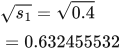 LaTeX:
\sqrt{s_1}=\sqrt{0.4}=0.632455532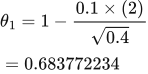 LaTeX:
\theta_1=1-\frac{0.1\times(2)}{\sqrt{0.4}}=0.683772234Step 2: Iteration 2 with supplied gradient 1.
Keep 90 percent of the old squared-gradient memory; add 10 percent of the new square.
 LaTeX:
s_2=0.9(0.4)+0.1(1)^2=0.46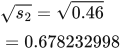 LaTeX:
\sqrt{s_2}=\sqrt{0.46}=0.678232998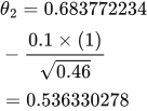 LaTeX:
\theta_2=0.683772234-\frac{0.1\times(1)}{\sqrt{0.46}}=0.536330278Drill 25 RMSProp variation 2
Question
Question. θ₀ = -0.5, η = 0.1, supplied successive gradients = [-1, 2]. Use RMSProp for two updates, zero initial accumulators and ε = 0 for this hand calculation. Use ρ = 0.9.
Answer — step by step
Given
Initial θ₀ = −0.5; η = 0.1.
Supplied gradients: [−1,2].
Initial accumulator(s) = 0; ε = 0 for this nonzero-denominator hand calculation.
ρ = 0.9.
To find
Find every stored state needed by the method and the parameter after each of two updates.
Formula — which one and why
RMSProp. Use a decaying average of squared gradients, then scale the current gradient by its square root. Old contributions gradually lose influence.
s = squared-gradient average; ρ (rho), sometimes written β, = retained fraction; g = current gradient; η = learning rate; ε = denominator stabilizer.
LaTeX: s_t=\rho s_{t-1}+(1-\rho)g_t^2LaTeX: \theta_t=\theta_{t-1}-\frac{\eta g_t}{\sqrt{s_t}+\epsilon}Yaad rakhne ka cue: Saare purane squares nahi—unki fading average.
Solution — step by step
Symbols and formulas used
θ is the parameter; η is the base learning rate; gₜ is the supplied gradient for update t. The gradients are already given, so no loss differentiation is needed here. Use ε = 0 only as specified in this exercise.
s is a moving average of squared gradients. ρ = 0.9 retains 90% of the old state; 1 − ρ = 0.1 supplies 10% of the new square. Start s₀ = 0.
LaTeX: s_t=\rho s_{t-1}+(1-\rho)g_t^2LaTeX: \theta_t=\theta_{t-1}-\frac{\eta g_t}{\sqrt{s_t}+\varepsilon}Use the supplied gradients in order. Initialize the stated memories to zero. Epsilon is set to zero only for this exercise because every denominator is nonzero. Keep calculator precision until the final result.
Step 1: Iteration 1 with supplied gradient -1.
Keep 90 percent of the old squared-gradient memory; add 10 percent of the new square.
 LaTeX:
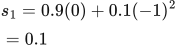
s_1=0.9(0)+0.1(-1)^2=0.1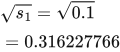 LaTeX:
\sqrt{s_1}=\sqrt{0.1}=0.316227766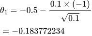 LaTeX:
\theta_1=-0.5-\frac{0.1\times(-1)}{\sqrt{0.1}}=-0.183772234Step 2: Iteration 2 with supplied gradient 2.
Keep 90 percent of the old squared-gradient memory; add 10 percent of the new square.
 LaTeX:
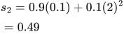
s_2=0.9(0.1)+0.1(2)^2=0.49 LaTeX:
\sqrt{s_2}=\sqrt{0.49}=0.7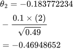 LaTeX:
\theta_2=-0.183772234-\frac{0.1\times(2)}{\sqrt{0.49}}=-0.46948652