Deep Learning · MT2 · formulas
Adam: correction and update
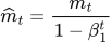
Adam starts its two averages at zero. Early averages therefore contain less total weight on observed gradients. Bias correction compensates for that initialization. The power in βᵗ uses the current update number, and both averages must be corrected before the parameter update.
 LaTeX:
\widehat m_t=\frac{m_t}{1-\beta_1^t} LaTeX:
\widehat v_t=\frac{v_t}{1-\beta_2^t}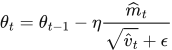 LaTeX:
\theta_t=\theta_{t-1}-\eta\frac{\widehat m_t}{\sqrt{\widehat v_t}+\epsilon}Adam bias correction: why the denominator is one minus beta to a power
Definition. Bias correction compensates for the reduced total observation weight caused by initializing an exponentially weighted accumulator to zero. Under a stationary gradient expectation, it removes the corresponding initialization bias in the moment estimate.
Explanation and working
1. What the moving average actually contains
Adam's signed-gradient memory is m. Starting with m₀ = 0 and β = 0.9, the first average is 90% of zero plus 10% of the first gradient. If g₁ = 2, then m₁ = 0.2. That small value partly reflects the artificial zero initialization.
 LaTeX:
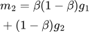
m_1=(1-\beta)g_1At the second step, substitute the first expression into the recurrence:
 LaTeX:
m_2=\beta(1-\beta)g_1+(1-\beta)g_22. Add the coefficients
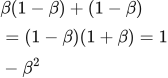
After the first step, the total coefficient attached to observed gradients is 1 − β. After two steps it is β(1 − β) + (1 − β). Factor out the common term:
 LaTeX:
\beta(1-\beta)+(1-\beta)=(1-\beta)(1+\beta)=1-\beta^2After t steps the coefficients sum to 1 − βᵗ. Dividing the stored average by that quantity removes this zero-start coefficient deficit.
LaTeX: \widehat m_t=\frac{m_t}{1-\beta_1^t}The squared-gradient memory uses its own decay β₂ and the same reasoning:
 LaTeX:
\widehat s_t=\frac{s_t}{1-\beta_2^t}3. A constant-gradient example makes the purpose visible
Let both gradients be 2 and use β₁ = 0.9. The first raw mean is 0.2; the second is 0.9 × 0.2 + 0.1 × 2 = 0.38.
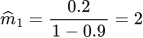 LaTeX:
\widehat m_1=\frac{0.2}{1-0.9}=2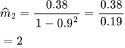 LaTeX:
\widehat m_2=\frac{0.38}{1-0.9^2}=\frac{0.38}{0.19}=2Both corrected values now equal the constant observed gradient. If gradients differ over time, the corrected result is a weighted average, not necessarily the latest gradient.
4. Two betas mean two separate powers
At update 2 with β₁ = 0.9 and β₂ = 0.999, the first correction denominator is 1 − 0.9² = 0.19. The second is 1 − 0.999² = 0.001999. Do not use 0.19 for both memories, and do not keep using the first-step denominators.
5. Correct first, then combine
The parameter update uses the corrected signed mean divided by the square root of the corrected squared mean, plus ε in the stated position. The square root is taken after correcting s. The numerator is not the loss, and no extra multiplication by g follows.
This derivation explains the formula; the following solved Adam examples show the complete arithmetic when gradients change sign or magnitude.
Adam remembers both direction and squared size
Definition. Adam, or adaptive moment estimation, uses bias-corrected exponentially weighted estimates of the first moment and the uncentered second moment of gradients to calculate parameter-specific updates.
What the two states represent
| State or coefficient | Meaning |
|---|---|
| mₜ | Moving average of signed gradients; retains directional information |
| sₜ | Moving average of squared gradients; estimates their uncentered second moment |
| β₁ | Decay coefficient for the first-moment estimate |
| β₂ | Decay coefficient for the second-moment estimate |
| t | Update number, starting at 1 for the first update |
| η and ε | Base learning rate and small denominator stabilizer |
The second moment is not the variance: it averages g² without subtracting a mean. Both states start at zero unless specified otherwise. These notes use s throughout this lesson; texts that use v for Adam's second moment mean the same state, not momentum's displacement velocity.
Recurrences, bias correction and update
 LaTeX:
m_t=\beta_1m_{t-1}+(1-\beta_1)g_t LaTeX:
s_t=\beta_2s_{t-1}+(1-\beta_2)g_t^2Zero initialization reduces the total weight initially attached to observed gradients. Divide by the appropriate accumulated observation weight:
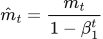 LaTeX:
\hat m_t=\frac{m_t}{1-\beta_1^t} LaTeX:
\hat s_t=\frac{s_t}{1-\beta_2^t}The update uses the corrected signed average in the numerator and the root of the corrected squared-gradient average in the denominator:
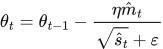 LaTeX:
\theta_t=\theta_{t-1}-\frac{\eta\hat m_t}{\sqrt{\hat s_t}+\varepsilon}The derivation in the next lesson explains why the correction factors contain powers of the iteration number. No additional multiplication by gₜ belongs in this final update: its contribution is already inside mₜ.
Complete numerical: changing gradient magnitude
Question. θ₀ = 1, m₀ = s₀ = 0, η = 0.1, β₁ = 0.9, β₂ = 0.999. Given g₁ = 2 and g₂ = 1, find two Adam updates, neglecting epsilon only in the numerical arithmetic.
Given
θ₀ = 1; initial state(s) = 0; η = 0.1.
Supplied gradients g₁ = 2, g₂ = 1.
ε = 0 for this hand calculation.
β₁ = 0.9; β₂ = 0.999; use bias correction.
To find
Calculate all required states and the parameter after each of two updates.
Formula — which one and why
Adam with bias correction. Keep two states: one averages signed gradients, the other averages squared gradients. Correct their initial bias toward zero before combining them in the parameter update.
m = signed average; s (also written v) = squared average; β₁ and β₂ = retained fractions; t = iteration number. A hat marks a corrected value. Carry raw m and s into the next recurrence.
LaTeX: m_t=\beta_1m_{t-1}+(1-\beta_1)g_tLaTeX: s_t=\beta_2s_{t-1}+(1-\beta_2)g_t^2LaTeX: \hat m_t=\frac{m_t}{1-\beta_1^t}LaTeX: \hat s_t=\frac{s_t}{1-\beta_2^t}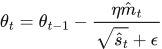 LaTeX:
\theta_t=\theta_{t-1}-\frac{\eta\hat m_t}{\sqrt{\hat s_t}+\epsilon}Yaad rakhne ka cue: Direction memory + square memory; hats lagao, phir update.
Solution — step by step
Iteration 1 — step 1: update the two raw states.
 LaTeX:
m_1=0.9(0)+0.1(2)=0.2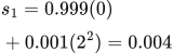 LaTeX:
s_1=0.999(0)+0.001(2^2)=0.004Step 2: correct both states using t = 1.
 LaTeX:
\hat m_1=\frac{0.2}{1-0.9^1}=\frac{0.2}{0.1}=2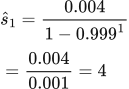 LaTeX:
\hat s_1=\frac{0.004}{1-0.999^1}=\frac{0.004}{0.001}=4Step 3: update the parameter.
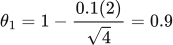 LaTeX:
\theta_1=1-\frac{0.1(2)}{\sqrt4}=0.9Start with the current gradient and the two states saved from the previous iteration.
Carry forward raw states: m = 0.2, s = 0.004. The corrected values are used for this update.
Iteration 2 — step 1: carry forward the raw states m₁ and s₁.
The recurrence uses the raw states 0.2 and 0.004, not the corrected values 2 and 4.
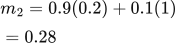 LaTeX:
m_2=0.9(0.2)+0.1(1)=0.28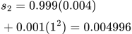 LaTeX:
s_2=0.999(0.004)+0.001(1^2)=0.004996Step 2: correct both states using t = 2.
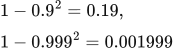 LaTeX:
1-0.9^2=0.19,\qquad1-0.999^2=0.001999 LaTeX:
\hat m_2=\frac{0.28}{0.19}\approx1.473684211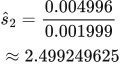 LaTeX:
\hat s_2=\frac{0.004996}{0.001999}\approx2.499249625Step 3: divide the corrected first moment by the corrected root.
 LaTeX:
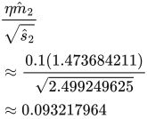
\frac{\eta\hat m_2}{\sqrt{\hat s_2}}\approx\frac{0.1(1.473684211)}{\sqrt{2.499249625}}\approx0.093217964Step 4: update from θ₁.
 LaTeX:
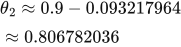
\theta_2\approx0.9-0.093217964\approx0.806782036Start with the current gradient and the two states saved from the previous iteration.
Carry forward raw states: m = 0.28, s = 0.004996. The corrected values are used for this update.
| State | After iteration 1 | After iteration 2 |
|---|---|---|
| Raw first moment m | 0.2 | 0.28 |
| Raw second moment s | 0.004 | 0.004996 |
| Corrected first moment | 2 | 1.473684211 |
| Corrected second moment | 4 | 2.499249625 |
| Parameter θ | 0.9 | 0.806782036 |
Final answer: θ₁ = 0.9 and θ₂ ≈ 0.806782. Store the raw moments for the next recurrence and use the corrected moments for the current parameter update.
Properties and limitations
Adam combines directional averaging with coordinate-specific scaling, which can be useful with noisy or differently scaled gradients. It requires two state values per parameter in addition to the parameter itself. η, β₁, β₂ and ε remain hyperparameters. Faster reduction of training loss does not establish better generalization, and Adam does not guarantee the global optimum of a general neural-network objective.
Drill 26 Adam variation 1
Question
Question. θ₀ = 1, η = 0.1, supplied successive gradients = [2, 1]. Use Adam for two updates, zero initial accumulators and ε = 0 for this hand calculation. Use β₁ = 0.9, β₂ = 0.999 and bias correction.
Answer — step by step
Given
Initial θ₀ = 1; η = 0.1.
Supplied gradients: [2,1].
Initial accumulator(s) = 0; ε = 0 for this nonzero-denominator hand calculation.
β₁ = 0.9; β₂ = 0.999; use bias correction.
To find
Find every stored state needed by the method and the parameter after each of two updates.
Formula — which one and why
Adam with bias correction. Keep two states: one averages signed gradients, the other averages squared gradients. Correct their initial bias toward zero before combining them in the parameter update.
m = signed average; s (also written v) = squared average; β₁ and β₂ = retained fractions; t = iteration number. A hat marks a corrected value. Carry raw m and s into the next recurrence.
LaTeX: m_t=\beta_1m_{t-1}+(1-\beta_1)g_tLaTeX: s_t=\beta_2s_{t-1}+(1-\beta_2)g_t^2LaTeX: \hat m_t=\frac{m_t}{1-\beta_1^t}LaTeX: \hat s_t=\frac{s_t}{1-\beta_2^t}LaTeX: \theta_t=\theta_{t-1}-\frac{\eta\hat m_t}{\sqrt{\hat s_t}+\epsilon}Yaad rakhne ka cue: Direction memory + square memory; hats lagao, phir update.
Solution — step by step
Symbols and formulas used
θ is the parameter; η is the base learning rate; gₜ is the supplied gradient for update t. The gradients are already given, so no loss differentiation is needed here. Use ε = 0 only as specified in this exercise.
m remembers signed gradients; v remembers squared gradients. The hats mean bias-corrected values, compensating for memories starting at zero. They are not extra powers. Here β₁ = 0.9 and β₂ = 0.999.
LaTeX: m_t=\beta_1m_{t-1}+(1-\beta_1)g_t LaTeX:
v_t=\beta_2v_{t-1}+(1-\beta_2)g_t^2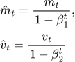 LaTeX:
\hat m_t=\frac{m_t}{1-\beta_1^t},\qquad \hat v_t=\frac{v_t}{1-\beta_2^t}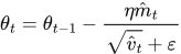 LaTeX:
\theta_t=\theta_{t-1}-\frac{\eta\hat m_t}{\sqrt{\hat v_t}+\varepsilon}Use the supplied gradients in order. Initialize the stated memories to zero. Epsilon is set to zero only for this exercise because every denominator is nonzero. Keep calculator precision until the final result.
Step 1: Iteration 1 with supplied gradient 2.
First calculate the signed-gradient mean m and squared-gradient mean v.
LaTeX: m_1=0.9(0)+0.1(2)=0.2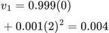 LaTeX:
v_1=0.999(0)+0.001(2)^2=0.004Correct each zero-initialized mean using this iteration number in the power.
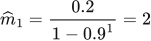 LaTeX:
\widehat m_1=\frac{0.2}{1-0.9^{1}}=2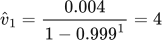 LaTeX:
\widehat v_1=\frac{0.004}{1-0.999^{1}}=4Divide the corrected direction by the corrected root, then subtract the scaled step.
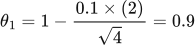 LaTeX:
\theta_1=1-\frac{0.1\times(2)}{\sqrt{4}}=0.9Step 2: Iteration 2 with supplied gradient 1.
First calculate the signed-gradient mean m and squared-gradient mean v.
LaTeX: m_2=0.9(0.2)+0.1(1)=0.28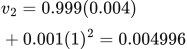 LaTeX:
v_2=0.999(0.004)+0.001(1)^2=0.004996Correct each zero-initialized mean using this iteration number in the power.
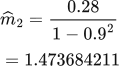 LaTeX:
\widehat m_2=\frac{0.28}{1-0.9^{2}}=1.473684211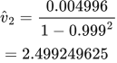 LaTeX:
\widehat v_2=\frac{0.004996}{1-0.999^{2}}=2.499249625Divide the corrected direction by the corrected root, then subtract the scaled step.
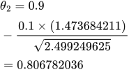 LaTeX:
\theta_2=0.9-\frac{0.1\times(1.473684211)}{\sqrt{2.499249625}}=0.806782036Drill 27 Adam variation 2
Question
Question. θ₀ = -0.5, η = 0.1, supplied successive gradients = [-1, 2]. Use Adam for two updates, zero initial accumulators and ε = 0 for this hand calculation. Use β₁ = 0.9, β₂ = 0.999 and bias correction.
Answer — step by step
Given
Initial θ₀ = −0.5; η = 0.1.
Supplied gradients: [−1,2].
Initial accumulator(s) = 0; ε = 0 for this nonzero-denominator hand calculation.
β₁ = 0.9; β₂ = 0.999; use bias correction.
To find
Find every stored state needed by the method and the parameter after each of two updates.
Formula — which one and why
Adam with bias correction. Keep two states: one averages signed gradients, the other averages squared gradients. Correct their initial bias toward zero before combining them in the parameter update.
m = signed average; s (also written v) = squared average; β₁ and β₂ = retained fractions; t = iteration number. A hat marks a corrected value. Carry raw m and s into the next recurrence.
LaTeX: m_t=\beta_1m_{t-1}+(1-\beta_1)g_tLaTeX: s_t=\beta_2s_{t-1}+(1-\beta_2)g_t^2LaTeX: \hat m_t=\frac{m_t}{1-\beta_1^t}LaTeX: \hat s_t=\frac{s_t}{1-\beta_2^t}LaTeX: \theta_t=\theta_{t-1}-\frac{\eta\hat m_t}{\sqrt{\hat s_t}+\epsilon}Yaad rakhne ka cue: Direction memory + square memory; hats lagao, phir update.
Solution — step by step
Symbols and formulas used
θ is the parameter; η is the base learning rate; gₜ is the supplied gradient for update t. The gradients are already given, so no loss differentiation is needed here. Use ε = 0 only as specified in this exercise.
m remembers signed gradients; v remembers squared gradients. The hats mean bias-corrected values, compensating for memories starting at zero. They are not extra powers. Here β₁ = 0.9 and β₂ = 0.999.
LaTeX: m_t=\beta_1m_{t-1}+(1-\beta_1)g_tLaTeX: v_t=\beta_2v_{t-1}+(1-\beta_2)g_t^2LaTeX: \hat m_t=\frac{m_t}{1-\beta_1^t},\qquad \hat v_t=\frac{v_t}{1-\beta_2^t}LaTeX: \theta_t=\theta_{t-1}-\frac{\eta\hat m_t}{\sqrt{\hat v_t}+\varepsilon}Use the supplied gradients in order. Initialize the stated memories to zero. Epsilon is set to zero only for this exercise because every denominator is nonzero. Keep calculator precision until the final result.
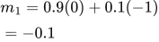
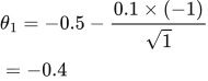
Step 1: Iteration 1 with supplied gradient -1.
First calculate the signed-gradient mean m and squared-gradient mean v.
 LaTeX:
m_1=0.9(0)+0.1(-1)=-0.1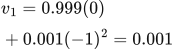 LaTeX:
v_1=0.999(0)+0.001(-1)^2=0.001Correct each zero-initialized mean using this iteration number in the power.
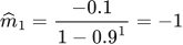 LaTeX:
\widehat m_1=\frac{-0.1}{1-0.9^{1}}=-1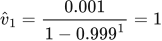 LaTeX:
\widehat v_1=\frac{0.001}{1-0.999^{1}}=1Divide the corrected direction by the corrected root, then subtract the scaled step.
 LaTeX:
\theta_1=-0.5-\frac{0.1\times(-1)}{\sqrt{1}}=-0.4Step 2: Iteration 2 with supplied gradient 2.
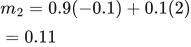
First calculate the signed-gradient mean m and squared-gradient mean v.
 LaTeX:
m_2=0.9(-0.1)+0.1(2)=0.11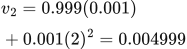 LaTeX:
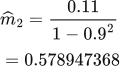
v_2=0.999(0.001)+0.001(2)^2=0.004999Correct each zero-initialized mean using this iteration number in the power.
 LaTeX:
\widehat m_2=\frac{0.11}{1-0.9^{2}}=0.578947368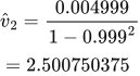 LaTeX:
\widehat v_2=\frac{0.004999}{1-0.999^{2}}=2.500750375Divide the corrected direction by the corrected root, then subtract the scaled step.
 LaTeX:
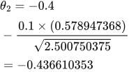
\theta_2=-0.4-\frac{0.1\times(0.578947368)}{\sqrt{2.500750375}}=-0.436610353