Deep Learning · MT2 · formulas
L1 penalty and update
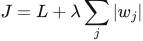
L1 adds a cost based on the absolute sizes of weights. Its derivative is positive for a positive weight and negative for a negative weight. The optimizer adds this penalty gradient to the data gradient before applying the usual update.
 LaTeX:
J=L+\lambda\sum_j|w_j| LaTeX:
w_{new}=w-\eta\left[g_{data}+\lambda\operatorname{sign}(w)\right]Model answer: regularization and the L1–L2 difference
Question
Question. What is regularization? Compare L1 and L2 regularization, including the objective, gradient effect and influence of regularization strength.
Answer — step by step
Regularization restricts or discourages certain fitted solutions to improve generalization. Weight penalties add a cost for parameter size to the training objective. The optimizer must balance fitting the data against that extra cost.
Objectives used in this course
 LaTeX:
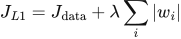
J_{L1}=J_{\mathrm{data}}+\lambda\sum_i|w_i|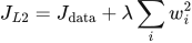 LaTeX:
J_{L2}=J_{\mathrm{data}}+\lambda\sum_iw_i^2Jdata measures prediction error. λ controls the strength of the additional penalty. The sums are over the weights included by the stated question.
| Basis | L1 | L2 |
|---|---|---|
| Quantity penalized | Absolute weight magnitude | Squared weight magnitude |
| Penalty derivative at nonzero w | λ sign(w) | 2λw under the displayed convention |
| Typical effect | Encourages sparse solutions | Smoothly shrinks weight magnitudes |
| Zero weights | Can promote exact zeros with suitable optimization | Usually leaves small nonzero weights |
The total gradient is the data-loss gradient plus the penalty gradient. With w = 2, data gradient 0.3 and λ = 0.1, the displayed L2 penalty adds 2 × 0.1 × 2 = 0.4. The total gradient is 0.7; update using that total.
Increasing λ strengthens the preference for smaller weights. Excessive regularization can prevent learning useful patterns and cause underfitting. L1 is not differentiable at zero, where a subgradient or suitable optimization method is used. If the examination writes λ/2 before the L2 sum, its penalty gradient becomes λw. Derive the factor from the printed objective.
L1 and L2 add a cost for large weights
Definition. Regularization modifies a training objective or learning procedure to constrain the fitted model and improve generalization. L1 and L2 regularization add parameter-norm penalties to the data loss.
Explanation and working
 LaTeX:
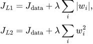
J_{L1}=J_{\mathrm{data}}+\lambda\sum_i|w_i|,\qquad J_{L2}=J_{\mathrm{data}}+\lambda\sum_iw_i^2Lambda controls how strongly you discourage weight size. L1 encourages sparsity, meaning many weights can become exactly zero under suitable optimization. L2 shrinks weights smoothly and usually leaves small nonzero values. Larger lambda can reduce overfitting, but excessive regularization can underfit.
Question. Data loss = 0.5; weights [2, −1]; λ = 0.1. Compute L1-regularized and L2-regularized objectives using the displayed convention.
Given
Data loss = 0.5; weights = [2,−1]; λ = 0.1.
The L2 convention here has no factor ½.
To find
Find L1/L2 penalties and the two regularized objective values.
Formula — which one and why
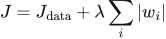
L1 penalty and gradient. Add absolute weight magnitudes to penalize large weights. Away from zero, the penalty derivative depends on the weight’s sign.
λ (lambda) = penalty strength; J_data = data loss; sign(w) is +1 for positive and −1 for negative weights. At zero a subgradient convention is needed.
 LaTeX:
J=J_{\mathrm{data}}+\lambda\sum_i|w_i| LaTeX:
g_i=g_{\mathrm{data},i}+\lambda\operatorname{sign}(w_i)Yaad rakhne ka cue: L1 absolute values leta hai; gradient mein sign aata hai.
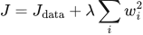
L2 penalty without a factor of one-half. This stated convention multiplies the sum of squares by λ, so differentiating contributes 2λw. Do not use the half-scaled gradient for this objective.
λ = penalty strength; J_data = original data loss; wᵢ = weight i.
 LaTeX:
J=J_{\mathrm{data}}+\lambda\sum_iw_i^2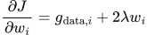 LaTeX:
\frac{\partial J}{\partial w_i}=g_{\mathrm{data},i}+2\lambda w_iYaad rakhne ka cue: Half nahi diya toh L2 derivative mein 2 lambda × weight.
Solution — step by step
Step 1: take absolute values for L1.
 LaTeX:
|2|=2,\qquad|-1|=1Step 2: add the absolute values.
 LaTeX:
2+1=3Step 3: multiply by lambda.
 LaTeX:
0.1(3)=0.3Step 4: add the data loss.
 LaTeX:
J_{L1}=0.5+0.3=0.8Step 5: square both weights for L2.
 LaTeX:
2^2=4,\qquad(-1)^2=1Step 6: add the squares.
 LaTeX:
4+1=5Step 7: multiply by lambda without adding a half.
 LaTeX:
0.1(5)=0.5Step 8: add the data loss.
 LaTeX:
J_{L2}=0.5+0.5=1.0For this L2 convention, the additional gradient is 2 λw. If the objective uses λ/2 times the squared sum, the additional gradient is λw instead. The factor is decided by the stated objective.
L2 gradient update without a half factor
Question. A weight is 2, its data-loss gradient is 0.3, λ = 0.1 and η = 0.01. The objective adds λw². Perform one update.
Given
w = 2; data gradient = 0.3; λ = 0.1; η = 0.01. The penalty has no factor ½.
To find
Penalty gradient, total gradient and updated weight.
Formula — which one and why
The derivative of λw² is 2λw. Add it to the data gradient before applying gradient descent.
λ is penalty strength; η is learning rate; g is the full objective gradient.
 LaTeX:
g_{\mathrm{penalty}}=2\lambda w LaTeX:
g=g_{\mathrm{data}}+g_{\mathrm{penalty}} LaTeX:
w_{\mathrm{new}}=w-\eta gYaad rakhne ka cue: Penalty ka gradient data gradient mein jodo, phir update.
Solution — step by step
Step 1: calculate the penalty gradient.
 LaTeX:
2(0.1)(2)=0.4Step 2: add the data gradient.
 LaTeX:
g=0.3+0.4=0.7Step 3: scale by the learning rate.
 LaTeX:
\eta g=0.01(0.7)=0.007Step 4: subtract from the old weight.
 LaTeX:
w_{\mathrm{new}}=2-0.007=1.993Final answer: Updated weight = 1.993. Bias penalties are omitted unless the objective includes them.
Deriving the L2 update
Under the objective written above, the data gradient and penalty gradient add:
 LaTeX:
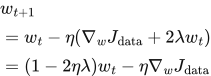
\nabla_w J=\nabla_w J_{\mathrm{data}}+2\lambda wFor ordinary gradient descent, regrouping the update gives:
 LaTeX:
w_{t+1}=w_t-\eta(\nabla_w J_{\mathrm{data}}+2\lambda w_t)=(1-2\eta\lambda)w_t-\eta\nabla_w J_{\mathrm{data}}This shows the shrinkage associated with this L2 convention. For an objective containing λ‖w‖²/2, replace 2λ by λ. This algebra explains the equivalence to appropriately scaled weight decay for ordinary gradient descent; adding an L2 term inside an adaptive optimizer is generally different from decoupled weight decay.
Drill 29 L1 update on positive and negative weights
Question
Question. w = [−0.5,0.3], data gradients = [0.2,−0.1], λ = 0.1, η = 0.2. Use L1 and ordinary gradient descent away from zero.
Answer — step by step
Given
Old weights = [−0.5,0.3].
Data gradients = [0.2,−0.1]; λ = 0.1; η = 0.2.
To find
Find total gradients and the two updated weights.
Formula — which one and why
L1 penalty and gradient. Add absolute weight magnitudes to penalize large weights. Away from zero, the penalty derivative depends on the weight’s sign.
λ (lambda) = penalty strength; J_data = data loss; sign(w) is +1 for positive and −1 for negative weights. At zero a subgradient convention is needed.
LaTeX: J=J_{\mathrm{data}}+\lambda\sum_i|w_i|LaTeX: g_i=g_{\mathrm{data},i}+\lambda\operatorname{sign}(w_i)Yaad rakhne ka cue: L1 absolute values leta hai; gradient mein sign aata hai.
Gradient descent. Evaluate the gradient at the current parameter, multiply by the learning rate and subtract. If the objective is supplied, differentiate it and recompute the gradient after each update.
θ (theta) = trainable parameter; g = derivative of the stated objective J; η = learning rate; t labels the update number.
 LaTeX:
g_t=J\prime(\theta_{t-1}) LaTeX:
\theta_t=\theta_{t-1}-\eta g_tYaad rakhne ka cue: Naya = purana − learning rate × current gradient.
Solution — step by step
Meaning and formula
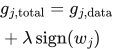
The supplied data gradient is only one part of the total gradient. L1 adds λ times the sign of the old weight. Sign is −1 for a negative weight and +1 for a positive weight.
 LaTeX:
g_{j,\mathrm{total}}=g_{j,\mathrm{data}}+\lambda\operatorname{sign}(w_j) LaTeX:
w_{j,\mathrm{new}}=w_j-\eta g_{j,\mathrm{total}}Both weights here are nonzero, so the ambiguous derivative of absolute value at zero is not needed.
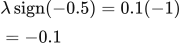
Step 1: Weight 1: old value −0.5.
 LaTeX:
\lambda\operatorname{sign}(-0.5)=0.1(-1)=-0.1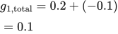 LaTeX:
g_{1,\mathrm{total}}=0.2+(-0.1)=0.1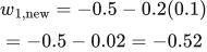 LaTeX:
w_{1,\mathrm{new}}=-0.5-0.2(0.1)=-0.5-0.02=-0.52Step 2: Weight 2: old value 0.3.
 LaTeX:
\lambda\operatorname{sign}(0.3)=0.1(1)=0.1 LaTeX:
g_{2,\mathrm{total}}=-0.1+0.1=0 LaTeX:
w_{2,\mathrm{new}}=0.3-0.2(0)=0.3Final answer: [−0.52, 0.3]. L1's own contribution pulls toward zero, but the combined data-plus-penalty update can move a weight away from zero.
Drill 28 Regularized objective
Question
Question. Data loss = 0.4, w = [−2,1,0.5], λ = 0.1. Calculate L1 objective and L2 objective using (λ/2)Σw².
Answer — step by step
Given
Data loss = 0.4; weights = [−2,1,0.5]; λ = 0.1.
For L2, the question includes the factor ½.
To find
Find each penalty and the total L1/L2 objective.
Formula — which one and why
L1 penalty and gradient. Add absolute weight magnitudes to penalize large weights. Away from zero, the penalty derivative depends on the weight’s sign.
λ (lambda) = penalty strength; J_data = data loss; sign(w) is +1 for positive and −1 for negative weights. At zero a subgradient convention is needed.
LaTeX: J=J_{\mathrm{data}}+\lambda\sum_i|w_i|LaTeX: g_i=g_{\mathrm{data},i}+\lambda\operatorname{sign}(w_i)Yaad rakhne ka cue: L1 absolute values leta hai; gradient mein sign aata hai.
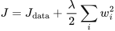
L2 penalty with a factor of one-half. Square each weight, sum and multiply by λ/2. The one-half cancels the factor 2 when differentiating, so the extra gradient is λw.
λ = penalty strength; w = old weight; J_data and g_data = data loss and its gradient.
 LaTeX:
J=J_{\mathrm{data}}+\frac\lambda2\sum_iw_i^2 LaTeX:
g_i=g_{\mathrm{data},i}+\lambda w_i LaTeX:
w_i^{\mathrm{new}}=w_i-\eta g_iYaad rakhne ka cue: Half wala L2 derivative mein lambda × weight deta hai.
Solution — step by step
Meaning and formulas
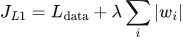
The data loss measures prediction error. A regularization penalty adds a cost for large weights. The objective J is the total being minimized. λ sets the strength of the penalty.
 LaTeX:
J_{L1}=L_{\mathrm{data}}+\lambda\sum_i|w_i|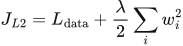 LaTeX:
J_{L2}=L_{\mathrm{data}}+\frac\lambda2\sum_iw_i^2Absolute value means ignore the sign. Squaring means multiply the number by itself. These are different operations.
Step 1: Part A: L1 objective.
 LaTeX:
|-2|=2,\quad |1|=1,\quad |0.5|=0.5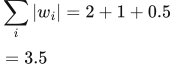 LaTeX:
\sum_i|w_i|=2+1+0.5=3.5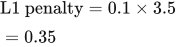 LaTeX:
\text{L1 penalty}=0.1\times3.5=0.35 LaTeX:
J_{L1}=0.4+0.35=0.75Step 2: Part B: L2 objective with the given half.
 LaTeX:
(-2)^2=4,\quad 1^2=1,\quad 0.5^2=0.25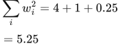 LaTeX:
\sum_iw_i^2=4+1+0.25=5.25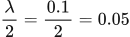 LaTeX:
\frac\lambda2=\frac{0.1}2=0.05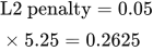 LaTeX:
\text{L2 penalty}=0.05\times5.25=0.2625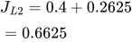 LaTeX:
J_{L2}=0.4+0.2625=0.6625Final answer: L1 objective 0.75; L2 objective 0.6625. These are total objectives, not just penalty values.
Drill 41 Mixed backpropagation and L2
Question
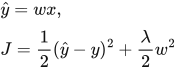
Question. Single linear neuron ŷ = wx, x = 2, w = 0.4, y = 1. Objective J = ½(ŷ−y)²+(λ/2)w², λ = 0.1, η = 0.2. Find loss, gradient, new weight.
Answer — step by step
Given
Prediction ŷ = wx; x = 2; w = 0.4; target y = 1.
Data loss = ½(ŷ−y)²; penalty = (λ/2)w².
λ = 0.1; η = 0.2.
To find
Find total objective, its weight gradient and the new weight.
Formula — which one and why
L2 penalty with a factor of one-half. Square each weight, sum and multiply by λ/2. The one-half cancels the factor 2 when differentiating, so the extra gradient is λw.
λ = penalty strength; w = old weight; J_data and g_data = data loss and its gradient.
LaTeX: J=J_{\mathrm{data}}+\frac\lambda2\sum_iw_i^2LaTeX: g_i=g_{\mathrm{data},i}+\lambda w_iLaTeX: w_i^{\mathrm{new}}=w_i-\eta g_iYaad rakhne ka cue: Half wala L2 derivative mein lambda × weight deta hai.
Gradient descent. Evaluate the gradient at the current parameter, multiply by the learning rate and subtract. If the objective is supplied, differentiate it and recompute the gradient after each update.
θ (theta) = trainable parameter; g = derivative of the stated objective J; η = learning rate; t labels the update number.
LaTeX: g_t=J\prime(\theta_{t-1})LaTeX: \theta_t=\theta_{t-1}-\eta g_tYaad rakhne ka cue: Naya = purana − learning rate × current gradient.
Solution — step by step
Meaning and formulas
This objective contains both prediction error and a weight penalty. Its gradient also has two parts. Compute both at the old weight, add them, then update once.
 LaTeX:
\hat y=wx,\qquad J=\frac12(\hat y-y)^2+\frac\lambda2w^2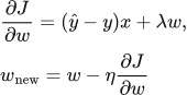 LaTeX:
\frac{\partial J}{\partial w}=(\hat y-y)x+\lambda w,\qquad w_{\mathrm{new}}=w-\eta\frac{\partial J}{\partial w}Step 1: prediction and error
 LaTeX:
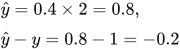
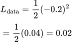
\hat y=0.4\times2=0.8,\qquad \hat y-y=0.8-1=-0.2Step 2: data loss
 LaTeX:
L_{\mathrm{data}}=\frac12(-0.2)^2=\frac12(0.04)=0.02Step 3: regularization penalty and total objective
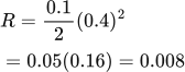 LaTeX:
R=\frac{0.1}{2}(0.4)^2=0.05(0.16)=0.008 LaTeX:
J=0.02+0.008=0.028Step 4: calculate the two gradient contributions
 LaTeX:
g_{\mathrm{data}}=(-0.2)\times2=-0.4 LaTeX:
g_{\mathrm{penalty}}=0.1\times0.4=0.04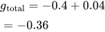 LaTeX:
g_{\mathrm{total}}=-0.4+0.04=-0.36Step 5: update
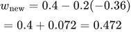 LaTeX:
w_{\mathrm{new}}=0.4-0.2(-0.36)=0.4+0.072=0.472Final answer: total loss 0.028; gradient −0.36; new weight 0.472.