F25 Q2b

Answer — step by step

A residual block learns a residual mapping F(x) and adds the input through a shortcut: y = F(x)+x, followed by an activation when the block design specifies one. A plain block without the shortcut outputs F(x). If F(x) becomes zero, the residual block can still pass x forward.

Diagram: The shortcut adds the input to the learned residual before the next stage. Labels: x | Learned layers F(x) | + | y | Shortcut S(x): identity or projection | y = F(x) + S(x) | S(x) = x for identity; S(x) = W_s x for projection. | Add matching shapes; do not concatenate.

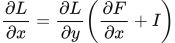LaTeX: \frac{\partial L}{\partial x}=\frac{\partial L}{\partial y}\left(\frac{\partial F}{\partial x}+I\right)

The identity term gives a direct gradient path. This helps optimize very deep networks and reduces the burden of learning an identity mapping through many nonlinear layers. Features can be reused or refined instead of being completely reconstructed by every block. Residual connections address optimization degradation and can help gradient flow, although they do not guarantee that vanishing gradients can never occur anywhere in the network.

Elementwise addition requires compatible shapes. If channel counts or spatial sizes differ, use a suitable projection shortcut, often a 1 × 1 convolution with the required stride. A shortcut is an addition, not channel concatenation. Example: x = [2,−1] and F(x) = [0.5,0.2] give y = [2.5,−0.8]; a subsequent ReLU gives [2.5,0]. Without the shortcut the preactivation output would be [0.5,0.2].

An Inception module captures features at multiple scales in parallel. A typical module has a 1 × 1 branch, a 1 × 1 reduction followed by 3 × 3 convolution, a 1 × 1 reduction followed by 5 × 5 convolution, and a pooling branch followed by 1 × 1 projection. Padding and strides preserve compatible spatial sizes so branch outputs can be concatenated along the channel axis.

Diagram: Parallel branches preserve height and width then concatenate channels. Labels: Input | 1 × 1 | 1 × 1 reduce | 3 × 3 | 1 × 1 reduce | 5 × 5 | 3 × 3 pool | 1 × 1 | Concatenate channels | All branch height/width values must match.

A 1 × 1 convolution mixes input channels at each position. With fewer output channels, it forms a bottleneck before an expensive larger kernel. ReLU following it adds nonlinearity. This reduces the number of input channels processed by 3 × 3 or 5 × 5 kernels while preserving useful learned combinations.

For H × W spatial size, Cin input channels and Cout output filters, a K × K convolution uses H × W × Cin × Cout × K² multiply-accumulates when the output spatial size stays H × W. A bottleneck changes the calculation to H × W × Cin × r + H × W × r × Cout × K². A multiply-accumulate is counted as one MAC here; some FLOP conventions count it as two operations. The benefit depends on the selected bottleneck width r. Compared with AlexNet's sequential kernels, Inception explicitly combines local and larger-scale features within one module.

AlexNet learns features along a mainly sequential stack of convolutional layers. Inception learns several spatial scales in parallel within a module and combines their channels. Both learn filter weights through backpropagation; their structural organization differs.