Deep Learning · MT2 · section
R26 Q5a
R26 selected MT2 practice
Question
Question (10 marks). Explain feedforward limitations for sequential context and how recurrence helps. Calculate h using tanh for Wxh is shown below, Whh is shown below, x = [0,1], hprevious = [0,1], zero bias. Explain next-word probabilities.
Answer — step by step
Given
Wxh and Whh are printed in the question; use their receiving-neuron rows.
Current input = [0,1]; previous hidden state = [0,1]; bias = 0.
Activation = tanh.
To find
Calculate both entries of the new hidden state. Output-layer weights are not supplied.
Formula — which one and why
Recurrent forward pass. At each time step, combine the current input contribution with the previous activated hidden state, add the bias and apply tanh. The same weights are reused at every time step.
x_t = current input; h_(t−1) = previous hidden state; W_xh = input weights; W_hh = recurrent weights; b = bias.
 LaTeX:
a_t=W_{xh}x_t+W_{hh}h_{t-1}+b LaTeX:
h_t=\tanh(a_t)Yaad rakhne ka cue: Naya input + pichhla activated state; phir activation.
Solution — step by step
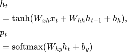
A recurrent neural network processes a sequence in order and maintains a hidden state that summarizes earlier information. Its weights are shared across time steps.
 LaTeX:
h_t=\tanh(W_{xh}x_t+W_{hh}h_{t-1}+b_h),\quad p_t=\operatorname{softmax}(W_{hy}h_t+b_y)At each step, transform the current token representation, transform the previous hidden state, add the bias and apply the activation. An output layer may produce a prediction at each step or only at the end. This allows a sequence's length to vary while the parameter set stays fixed.
For next-word prediction, tokenize text, represent each word numerically, update the state for each prefix token, and apply an output softmax over the vocabulary. Train against the actual next token using cross-entropy. For sentiment classification, use the sequence representation to predict positive, neutral or negative. Word order matters: “not good” should not be interpreted like “good”.
A basic feedforward model has no built-in recurrent state, though a fixed window can be supplied explicitly. RNNs provide recurrent context but have sequential computation costs and difficulty learning long dependencies because of vanishing or exploding gradients. An encoder-decoder RNN can encode a source sentence and generate a target sentence of a different length; this is a historical RNN translation explanation, not a claim about any commercial service's current architecture.
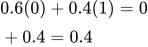
Step 1: multiply the input vector into row 1.
 LaTeX:
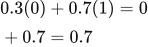
0.6(0)+0.4(1)=0+0.4=0.4Step 2: multiply the input vector into row 2.
 LaTeX:
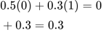
0.3(0)+0.7(1)=0+0.7=0.7Step 3: multiply previous state into recurrent row 1.
 LaTeX:
0.5(0)+0.3(1)=0+0.3=0.3Step 4: multiply previous state into recurrent row 2.
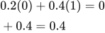 LaTeX:
0.2(0)+0.4(1)=0+0.4=0.4Step 5: combine contributions for hidden unit 1.
 LaTeX:
a_1=0.4+0.3+0=0.7Step 6: combine contributions for hidden unit 2.
 LaTeX:
a_2=0.7+0.4+0=1.1Step 7: apply tanh separately to each complete sum.
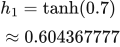 LaTeX:
h_1=\tanh(0.7)\approx0.604367777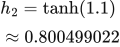 LaTeX:
h_2=\tanh(1.1)\approx0.800499022Final answer: h ≈ [0.604367777,0.800499022]. The absent vocabulary output weights prevent calculating a numerical next-word probability list.