Deep Learning · MT2 · section
F22 Q3b
F22 selected MT2 practice
Question
Question (10 marks). Count trainable parameters of the illustrated LeNet-style digit classifier with convolution 5 × 5: 6 filters, pooling 2; convolution 5 × 5: 16 filters, pooling 2; dense 120, dense 84, softmax 10. Use the consistent 32 × 32 × 1 input that produces the drawn 28,14,10,5 spatial maps.
Answer — step by step
Given
Count trainable parameters of the illustrated LeNet-style digit classifier with convolution 5 × 5: 6 filters, pooling 2.
convolution 5 × 5: 16 filters, pooling 2.
dense 120, dense 84, softmax 10.
Use the consistent 32 × 32 × 1 input that produces the drawn 28,14,10,5 spatial maps.
To find
Find every layer shape, its parameter count and the network total.
Formula — which one and why
Complete CNN calculation. Carry each output shape into the next layer. Convolution changes spatial size and channel count; pooling changes spatial size; flattening converts all activations into dense-layer inputs.
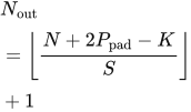
H,W,C = feature-map height, width and channels; K = kernel size; S = stride; P_pad = padding. One bias is assumed for each learned filter or dense neuron unless specified otherwise.
 LaTeX:
N_{\mathrm{out}}=\left\lfloor\frac{N+2P_{\mathrm{pad}}-K}{S}\right\rfloor+1 LaTeX:
P_{\mathrm{conv}}=(K^2C_{\mathrm{in}}+1)C_{\mathrm{out}} LaTeX:
n_{\mathrm{flat}}=HWC LaTeX:
P_{\mathrm{dense}}=(n_{\mathrm{in}}+1)n_{\mathrm{out}} LaTeX:
P_{\mathrm{pool}}=P_{\mathrm{flatten}}=0Yaad rakhne ka cue: Ek layer ka output, next layer ka input; shape aur parameters alag count.
Solution — step by step
Use output size 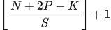 LaTeX:
\left\lfloor\frac{N+2P-K}{S}\right\rfloor+1, Conv weights K² × Cin × Cout and biases Cout, Dense weights Nin × Nout and biases Nout. Assume a bias per learned filter/unit, full input-channel connectivity and no trainable pooling parameters. ReLU and softmax activations themselves add no trainable parameters.
Layer-by-layer calculation
Carry the complete output shape of one layer into the next. Spatial size determines the number of activations; it does not multiply the number of shared convolution parameters.
Layer 1 — convolution
Spatial positions share the filter weights. Output depth equals the number of filters.
Input: 32 × 32 × 1. Use 6 filters of spatial size 5 × 5, stride 1, and padding 0 on each side.
1. Calculate height and width.
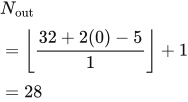 LaTeX:
N_{\mathrm{out}}=\left\lfloor\frac{32+2(0)-5}{1}\right\rfloor+1=282. Determine output channels. Each filter produces one feature map. Therefore the output is 28 × 28 × 6.
3. Count trainable values. Each filter receives all 1 input channels. Its weights are reused at every spatial position.
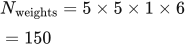 LaTeX:
N_{\mathrm{weights}}=5\times5\times1\times6=150 LaTeX:
N_{\mathrm{biases}}=6 LaTeX:
P_1=150+6=156Layer 2 — pooling
Spatial dimensions change; the channel count stays the same. Pooling learns no weights.
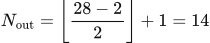
Input: 28 × 28 × 6. Use a 2 × 2 window, stride 2, and zero padding.
 LaTeX:
N_{\mathrm{out}}=\left\lfloor\frac{28-2}{2}\right\rfloor+1=14Pooling acts independently on each channel. The output is 14 × 14 × 6.
Trainable parameters: 0. Max/average pooling has no learned filter weights or biases.
Layer 3 — convolution
Spatial positions share the filter weights. Output depth equals the number of filters.
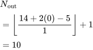
Input: 14 × 14 × 6. Use 16 filters of spatial size 5 × 5, stride 1, and padding 0 on each side.
1. Calculate height and width.
 LaTeX:
N_{\mathrm{out}}=\left\lfloor\frac{14+2(0)-5}{1}\right\rfloor+1=102. Determine output channels. Each filter produces one feature map. Therefore the output is 10 × 10 × 16.
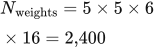
3. Count trainable values. Each filter receives all 6 input channels. Its weights are reused at every spatial position.
 LaTeX:
N_{\mathrm{weights}}=5\times5\times6\times16=2{,}400 LaTeX:
N_{\mathrm{biases}}=16 LaTeX:
P_3=2{,}400+16=2{,}416Layer 4 — pooling
Spatial dimensions change; the channel count stays the same. Pooling learns no weights.
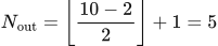
Input: 10 × 10 × 16. Use a 2 × 2 window, stride 2, and zero padding.
 LaTeX:
N_{\mathrm{out}}=\left\lfloor\frac{10-2}{2}\right\rfloor+1=5Pooling acts independently on each channel. The output is 5 × 5 × 16.
Trainable parameters: 0. Max/average pooling has no learned filter weights or biases.
Layer 5 — flatten
The same activation values are rearranged into one vector. No parameter is learned.
Input: 5 × 5 × 16. Rearrange all activation values into one vector.
 LaTeX:
n_{\mathrm{flat}}=5\times5\times16=400Output: a vector with 400 entries. Flattening changes the arrangement, so it adds 0 trainable parameters.
Layer 6 — fully connected layer
Every output neuron receives every input feature, with one bias per output neuron.
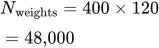
Input: 400 features. Output: 120 neurons. Every output neuron connects to every input feature and has one bias.
 LaTeX:
N_{\mathrm{weights}}=400\times120=48{,}000 LaTeX:
N_{\mathrm{biases}}=120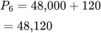 LaTeX:
P_6=48{,}000+120=48{,}120Layer 7 — fully connected layer
Every output neuron receives every input feature, with one bias per output neuron.
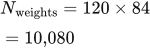
Input: 120 features. Output: 84 neurons. Every output neuron connects to every input feature and has one bias.
 LaTeX:
N_{\mathrm{weights}}=120\times84=10{,}080 LaTeX:
N_{\mathrm{biases}}=84 LaTeX:
P_7=10{,}080+84=10{,}164Layer 8 — fully connected layer
Every output neuron receives every input feature, with one bias per output neuron.
Input: 84 features. Output: 10 neurons. Every output neuron connects to every input feature and has one bias.
 LaTeX:
N_{\mathrm{weights}}=84\times10=840 LaTeX:
N_{\mathrm{biases}}=10 LaTeX:
P_8=840+10=850Summary of the complete network
| Layer | Spatial or flatten calculation | Output | Weights | Biases | Total |
|---|---|---|---|---|---|
| 1 conv | 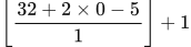 LaTeX: \left\lfloor\frac{32+2 \times 0-5}{1}\right\rfloor+1 | 28 x 28 x 6 | 150 | 6 | 156 |
| 2 pool | 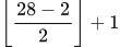 LaTeX: \left\lfloor\frac{28-2}{2}\right\rfloor+1 | 14 x 14 x 6 | 0 | 0 | 0 |
| 3 conv | 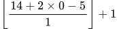 LaTeX: \left\lfloor\frac{14+2 \times 0-5}{1}\right\rfloor+1 | 10 x 10 x 16 | 2,400 | 16 | 2,416 |
| 4 pool | 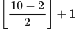 LaTeX: \left\lfloor\frac{10-2}{2}\right\rfloor+1 | 5 x 5 x 16 | 0 | 0 | 0 |
| 5 flat | 5 × 5 × 16 | 400 | 0 | 0 | 0 |
| 6 dense | 400 → 120 | 120 | 48,000 | 120 | 48,120 |
| 7 dense | 120 → 84 | 84 | 10,080 | 84 | 10,164 |
| 8 dense | 84 → 10 | 10 | 840 | 10 | 850 |
Parameter substitutions, in layer order:
Layer 1: (5 x 5 x 1 + 1) x 6 = 156.
Layer 3: (5 x 5 x 6 + 1) x 16 = 2,416.
Layer 6: (400 + 1) x 120 = 48,120.
Layer 7: (120 + 1) x 84 = 10,164.
Layer 8: (84 + 1) x 10 = 850.
Total: 156 + 2,416 + 48,120 + 10,164 + 850 = 61,706 trainable parameters. Pooling changes activation size; it does not itself add learned weights. Always floor noninteger spatial dimensions.
This is the standard classroom full-channel interpretation with nontrainable pooling and a dense 10-class softmax. The historical original LeNet used partial channel connections and other details, so its published parameter count need not equal this diagram-based count. If an input label is read as 28, the stated later 28 map after valid 5 × 5 convolution is inconsistent; record the 32 input assumption rather than silently ignoring the mismatch.