Drill 14 Batch and sequential SGD

Answer — step by step

Given

Model ŷ = wx; initial w = 0; η = 0.1.

Samples in order: (x,y) = (1,1), then (2,2).

Batch objective: mean half squared loss.

To find

Compare the weight after one batch update and one sequential SGD epoch.

Formula — which one and why

Batch mean versus sequential SGD. A batch update averages gradients evaluated at the same old parameter. Sequential SGD updates after each sample, so later samples use the changed parameter.

B = number of examples in the batch; gᵢ = sample gradient; η = learning rate. For the linear half squared objective, sample gradient is (wx−y)x.

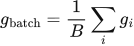LaTeX: g_{\mathrm{batch}}=\frac1B\sum_i g_i

LaTeX: g_i=(wx_i-y_i)x_i

LaTeX: w_{\mathrm{new}}=w-\eta g

Yaad rakhne ka cue: Batch: same old weight par average; SGD: har sample ke baad weight change.

Solution — step by step

Meaning and formulas

For one sample, x is the input, y is the target, and w is the weight. Batch GD averages gradients evaluated at the same old weight. Sequential SGD updates after each sample and uses that new weight for the next sample.

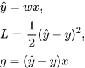LaTeX: \hat y=wx,\quad L=\frac12(\hat y-y)^2,\quad g=(\hat y-y)x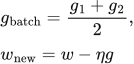

LaTeX: g_{\mathrm{batch}}=\frac{g_1+g_2}{2},\qquad w_{\mathrm{new}}=w-\eta g

Step 1: Part A: one batch update from w = 0.

For sample (1,1), prediction = 0 × 1 = 0, so:

LaTeX: g_1=(0-1)\times1=-1

For sample (2,2), keep the same weight 0. Prediction = 0 × 2 = 0, so:

LaTeX: g_2=(0-2)\times2=-4

Average these two gradients, then update once.

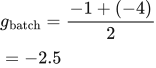LaTeX: g_{\mathrm{batch}}=\frac{-1+(-4)}2=-2.5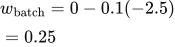

LaTeX: w_{\mathrm{batch}}=0-0.1(-2.5)=0.25

Step 2: Part B: one SGD epoch, restarting at w = 0.

The first sample has gradient −1, just as above.

LaTeX: w_1=0-0.1(-1)=0.1

For the second sample use this new weight, so prediction is:

LaTeX: \hat y_2=0.1\times2=0.2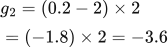

LaTeX: g_2=(0.2-2)\times2=(-1.8)\times2=-3.6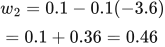

LaTeX: w_2=0.1-0.1(-3.6)=0.1+0.36=0.46

Final answer: batch result 0.25; sequential SGD result 0.46. The difference comes from the timing of the updates.