Deep Learning · MT2 · section
Drill 32 Convolution with a negative coefficient
MT2 numerical practice from direct to mixed
Question
Question. Use the input A and kernel K shown below, stride 1, padding 0. Compute all outputs.
| 1 | 2 | 0 | 1 |
| 0 | 1 | 3 | 2 |
| 2 | 1 | 0 | 1 |
| 1 | 0 | 2 | 3 |
| 1 | −1 |
| 0 | 1 |
Stride 1; P = 0 (no padding).
Answer — step by step
Given
Input A and kernel K are printed with the question.
Stride S = 1; padding P = 0; bias = 0.
Use the kernel without flipping it.
To find
Calculate all nine output cells.
Formula — which one and why
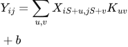
Convolution values. At each valid location, multiply corresponding window and kernel entries, add all products and add the filter bias once. Move by the stated stride and repeat.
X = input; K = kernel; S = stride; b = filter bias; u,v locate a kernel entry. Use the printed kernel without flipping under the stated deep-learning convention.
 LaTeX:
Y_{ij}=\sum_{u,v}X_{iS+u,jS+v}K_{uv}+bYaad rakhne ka cue: Matching cells multiply; sab products add; bias sirf ek baar.
Solution — step by step
Formulas and the operation we are performing
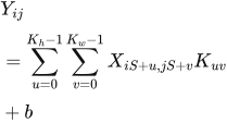
A filter window produces one output value. Multiply entries at matching positions and add the products. In this deep-learning convention, keep the filter in its printed orientation.
 LaTeX:
Y_{ij}=\sum_{u=0}^{K_h-1}\sum_{v=0}^{K_w-1}X_{iS+u,jS+v}K_{uv}+bHere i and j identify an output position; u and v count positions inside its window. S is stride, and b is the filter bias, zero in this question. The equation uses a padded input if padding is present and zero-based indices; the working below labels output positions from 1 for readability.
 LaTeX:
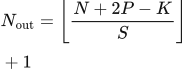
N_{\mathrm{out}}=\left\lfloor\frac{N+2P-K}{S}\right\rfloor+1N is input width/height, P is padding per side, and K is filter width/height. Floor means take the integer below the result, then add one.
Follow each selected input window below. Matching row colors connect its input cells, kernel coefficients and products; the outlined output cell shows where their sum belongs.
Step 1 shape: 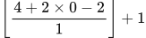 LaTeX:
\left\lfloor\frac{4+2 \times 0-2}{1}\right\rfloor+1 = 3 along each axis. Use the deep-learning cross-correlation convention: do not flip the printed kernel.
Output position (1, 1)
Use this position's input window. Multiply corresponding entries row by row; then add all row totals.
Input rows 1–2, columns 1–2. The window moves 1 cell per output step.
| 1 | 2 | 0 | 1 |
| 0 | 1 | 3 | 2 |
| 2 | 1 | 0 | 1 |
| 1 | 0 | 2 | 3 |
Only the outlined cells belong to this output.
| 1 | −1 |
| 0 | 1 |
Same row and column positions; no matrix multiplication.
| 1 | −2 |
| 0 | 1 |
Each cell is input × matching kernel coefficient.
(−1) + 1 = 0
| 0 | 5 | 1 |
| 0 | −2 | 2 |
| 1 | 3 | 2 |
Output row 1, column 1.
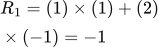
Window row 1.
 LaTeX:
R_1=(1)\times(1)+(2)\times(-1)=-1Window row 2.
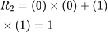 LaTeX:
R_2=(0)\times(0)+(1)\times(1)=1Add the rows to obtain one output cell.
 LaTeX:
Y_{1,1}=(-1)+(1)=0Output position (1, 2)
Use this position's input window. Multiply corresponding entries row by row; then add all row totals.
Input rows 1–2, columns 2–3. The window moves 1 cell per output step.
| 1 | 2 | 0 | 1 |
| 0 | 1 | 3 | 2 |
| 2 | 1 | 0 | 1 |
| 1 | 0 | 2 | 3 |
Only the outlined cells belong to this output.
| 1 | −1 |
| 0 | 1 |
Same row and column positions; no matrix multiplication.
| 2 | 0 |
| 0 | 3 |
Each cell is input × matching kernel coefficient.
2 + 3 = 5
| 0 | 5 | 1 |
| 0 | −2 | 2 |
| 1 | 3 | 2 |
Output row 1, column 2.
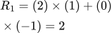
Window row 1.
 LaTeX:
R_1=(2)\times(1)+(0)\times(-1)=2Window row 2.
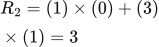 LaTeX:
R_2=(1)\times(0)+(3)\times(1)=3Add the rows to obtain one output cell.
 LaTeX:
Y_{1,2}=(2)+(3)=5Output position (1, 3)
Use this position's input window. Multiply corresponding entries row by row; then add all row totals.
Input rows 1–2, columns 3–4. The window moves 1 cell per output step.
| 1 | 2 | 0 | 1 |
| 0 | 1 | 3 | 2 |
| 2 | 1 | 0 | 1 |
| 1 | 0 | 2 | 3 |
Only the outlined cells belong to this output.
| 1 | −1 |
| 0 | 1 |
Same row and column positions; no matrix multiplication.
| 0 | −1 |
| 0 | 2 |
Each cell is input × matching kernel coefficient.
(−1) + 2 = 1
| 0 | 5 | 1 |
| 0 | −2 | 2 |
| 1 | 3 | 2 |
Output row 1, column 3.
Window row 1.
 LaTeX:
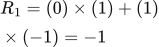
R_1=(0)\times(1)+(1)\times(-1)=-1Window row 2.
 LaTeX:
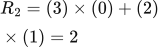
R_2=(3)\times(0)+(2)\times(1)=2Add the rows to obtain one output cell.
 LaTeX:
Y_{1,3}=(-1)+(2)=1Output position (2, 1)
Use this position's input window. Multiply corresponding entries row by row; then add all row totals.
Input rows 2–3, columns 1–2. The window moves 1 cell per output step.
| 1 | 2 | 0 | 1 |
| 0 | 1 | 3 | 2 |
| 2 | 1 | 0 | 1 |
| 1 | 0 | 2 | 3 |
Only the outlined cells belong to this output.
| 1 | −1 |
| 0 | 1 |
Same row and column positions; no matrix multiplication.
| 0 | −1 |
| 0 | 1 |
Each cell is input × matching kernel coefficient.
(−1) + 1 = 0
| 0 | 5 | 1 |
| 0 | −2 | 2 |
| 1 | 3 | 2 |
Output row 2, column 1.
Window row 1.
LaTeX: R_1=(0)\times(1)+(1)\times(-1)=-1Window row 2.
 LaTeX:
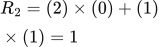
R_2=(2)\times(0)+(1)\times(1)=1Add the rows to obtain one output cell.
 LaTeX:
Y_{2,1}=(-1)+(1)=0Output position (2, 2)
Use this position's input window. Multiply corresponding entries row by row; then add all row totals.
Input rows 2–3, columns 2–3. The window moves 1 cell per output step.
| 1 | 2 | 0 | 1 |
| 0 | 1 | 3 | 2 |
| 2 | 1 | 0 | 1 |
| 1 | 0 | 2 | 3 |
Only the outlined cells belong to this output.
| 1 | −1 |
| 0 | 1 |
Same row and column positions; no matrix multiplication.
| 1 | −3 |
| 0 | 0 |
Each cell is input × matching kernel coefficient.
(−2) + 0 = −2
| 0 | 5 | 1 |
| 0 | −2 | 2 |
| 1 | 3 | 2 |
Output row 2, column 2.
Window row 1.
 LaTeX:
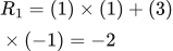
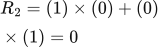
R_1=(1)\times(1)+(3)\times(-1)=-2Window row 2.
 LaTeX:
R_2=(1)\times(0)+(0)\times(1)=0Add the rows to obtain one output cell.
 LaTeX:
Y_{2,2}=(-2)+(0)=-2Output position (2, 3)
Use this position's input window. Multiply corresponding entries row by row; then add all row totals.
Input rows 2–3, columns 3–4. The window moves 1 cell per output step.
| 1 | 2 | 0 | 1 |
| 0 | 1 | 3 | 2 |
| 2 | 1 | 0 | 1 |
| 1 | 0 | 2 | 3 |
Only the outlined cells belong to this output.
| 1 | −1 |
| 0 | 1 |
Same row and column positions; no matrix multiplication.
| 3 | −2 |
| 0 | 1 |
Each cell is input × matching kernel coefficient.
1 + 1 = 2
| 0 | 5 | 1 |
| 0 | −2 | 2 |
| 1 | 3 | 2 |
Output row 2, column 3.
Window row 1.
 LaTeX:
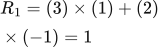
R_1=(3)\times(1)+(2)\times(-1)=1Window row 2.
LaTeX: R_2=(0)\times(0)+(1)\times(1)=1Add the rows to obtain one output cell.
 LaTeX:
Y_{2,3}=(1)+(1)=2Output position (3, 1)
Use this position's input window. Multiply corresponding entries row by row; then add all row totals.
Input rows 3–4, columns 1–2. The window moves 1 cell per output step.
| 1 | 2 | 0 | 1 |
| 0 | 1 | 3 | 2 |
| 2 | 1 | 0 | 1 |
| 1 | 0 | 2 | 3 |
Only the outlined cells belong to this output.
| 1 | −1 |
| 0 | 1 |
Same row and column positions; no matrix multiplication.
| 2 | −1 |
| 0 | 0 |
Each cell is input × matching kernel coefficient.
1 + 0 = 1
| 0 | 5 | 1 |
| 0 | −2 | 2 |
| 1 | 3 | 2 |
Output row 3, column 1.
Window row 1.
 LaTeX:
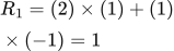
R_1=(2)\times(1)+(1)\times(-1)=1Window row 2.
LaTeX: R_2=(1)\times(0)+(0)\times(1)=0Add the rows to obtain one output cell.
 LaTeX:
Y_{3,1}=(1)+(0)=1Output position (3, 2)
Use this position's input window. Multiply corresponding entries row by row; then add all row totals.
Input rows 3–4, columns 2–3. The window moves 1 cell per output step.
| 1 | 2 | 0 | 1 |
| 0 | 1 | 3 | 2 |
| 2 | 1 | 0 | 1 |
| 1 | 0 | 2 | 3 |
Only the outlined cells belong to this output.
| 1 | −1 |
| 0 | 1 |
Same row and column positions; no matrix multiplication.
| 1 | 0 |
| 0 | 2 |
Each cell is input × matching kernel coefficient.
1 + 2 = 3
| 0 | 5 | 1 |
| 0 | −2 | 2 |
| 1 | 3 | 2 |
Output row 3, column 2.
Window row 1.
 LaTeX:
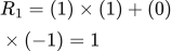
R_1=(1)\times(1)+(0)\times(-1)=1Window row 2.
 LaTeX:
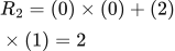
R_2=(0)\times(0)+(2)\times(1)=2Add the rows to obtain one output cell.
 LaTeX:
Y_{3,2}=(1)+(2)=3Output position (3, 3)
Use this position's input window. Multiply corresponding entries row by row; then add all row totals.
Input rows 3–4, columns 3–4. The window moves 1 cell per output step.
| 1 | 2 | 0 | 1 |
| 0 | 1 | 3 | 2 |
| 2 | 1 | 0 | 1 |
| 1 | 0 | 2 | 3 |
Only the outlined cells belong to this output.
| 1 | −1 |
| 0 | 1 |
Same row and column positions; no matrix multiplication.
| 0 | −1 |
| 0 | 3 |
Each cell is input × matching kernel coefficient.
(−1) + 3 = 2
| 0 | 5 | 1 |
| 0 | −2 | 2 |
| 1 | 3 | 2 |
Output row 3, column 3.
Window row 1.
LaTeX: R_1=(0)\times(1)+(1)\times(-1)=-1Window row 2.
 LaTeX:
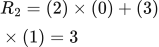
R_2=(2)\times(0)+(3)\times(1)=3Add the rows to obtain one output cell.
 LaTeX:
Y_{3,3}=(-1)+(3)=2Final output: 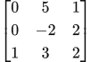 LaTeX:
\begin{bmatrix}0 & 5 & 1\\0 & -2 & 2\\1 & 3 & 2\end{bmatrix}. Each output came from its own complete window; stride changes the next window position, not the multiplication rule.