Deep Learning · MT2 · section
Drill 41 Mixed backpropagation and L2
MT2 numerical practice from direct to mixed
Question
Question. Single linear neuron ŷ = wx, x = 2, w = 0.4, y = 1. Objective J = ½(ŷ−y)²+(λ/2)w², λ = 0.1, η = 0.2. Find loss, gradient, new weight.
Answer — step by step
Given
Prediction ŷ = wx; x = 2; w = 0.4; target y = 1.
Data loss = ½(ŷ−y)²; penalty = (λ/2)w².
λ = 0.1; η = 0.2.
To find
Find total objective, its weight gradient and the new weight.
Formula — which one and why
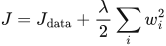
L2 penalty with a factor of one-half. Square each weight, sum and multiply by λ/2. The one-half cancels the factor 2 when differentiating, so the extra gradient is λw.
λ = penalty strength; w = old weight; J_data and g_data = data loss and its gradient.
 LaTeX:
J=J_{\mathrm{data}}+\frac\lambda2\sum_iw_i^2 LaTeX:
g_i=g_{\mathrm{data},i}+\lambda w_i LaTeX:
w_i^{\mathrm{new}}=w_i-\eta g_iYaad rakhne ka cue: Half wala L2 derivative mein lambda × weight deta hai.
Gradient descent. Evaluate the gradient at the current parameter, multiply by the learning rate and subtract. If the objective is supplied, differentiate it and recompute the gradient after each update.
θ (theta) = trainable parameter; g = derivative of the stated objective J; η = learning rate; t labels the update number.
 LaTeX:
g_t=J\prime(\theta_{t-1}) LaTeX:
\theta_t=\theta_{t-1}-\eta g_tYaad rakhne ka cue: Naya = purana − learning rate × current gradient.
Solution — step by step
Meaning and formulas
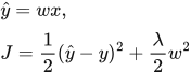
This objective contains both prediction error and a weight penalty. Its gradient also has two parts. Compute both at the old weight, add them, then update once.
 LaTeX:
\hat y=wx,\qquad J=\frac12(\hat y-y)^2+\frac\lambda2w^2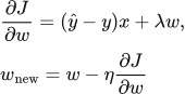 LaTeX:
\frac{\partial J}{\partial w}=(\hat y-y)x+\lambda w,\qquad w_{\mathrm{new}}=w-\eta\frac{\partial J}{\partial w}Step 1: prediction and error
 LaTeX:
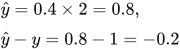
\hat y=0.4\times2=0.8,\qquad \hat y-y=0.8-1=-0.2Step 2: data loss
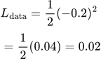 LaTeX:
L_{\mathrm{data}}=\frac12(-0.2)^2=\frac12(0.04)=0.02Step 3: regularization penalty and total objective
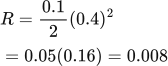 LaTeX:
R=\frac{0.1}{2}(0.4)^2=0.05(0.16)=0.008 LaTeX:
J=0.02+0.008=0.028Step 4: calculate the two gradient contributions
 LaTeX:
g_{\mathrm{data}}=(-0.2)\times2=-0.4 LaTeX:
g_{\mathrm{penalty}}=0.1\times0.4=0.04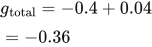 LaTeX:
g_{\mathrm{total}}=-0.4+0.04=-0.36Step 5: update
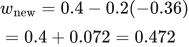 LaTeX:
w_{\mathrm{new}}=0.4-0.2(-0.36)=0.4+0.072=0.472Final answer: total loss 0.028; gradient −0.36; new weight 0.472.