Deep Learning · MT2 · section
Drill 6 Chain rule on a tiny loss
MT2 numerical practice from direct to mixed
Question
Question. Let o = wx+b, L = ½(o−y)², x = 3, w = 0.2, b = 0.1, y = 1. Find dL/dw, dL/db and update at η = 0.1.
Answer — step by step
Given
Model: o = wx+b; loss L = ½(o−y)².
x = 3; y = 1; w = 0.2; b = 0.1.
Learning rate η = 0.1.
To find
Find ∂L/∂w, ∂L/∂b and the updated weight and bias.
Formula — which one and why
Chain rule for a linear neuron. The weight changes the prediction, and the prediction changes the loss. Multiply those two local rates. Half squared loss differentiates to prediction minus target; the neuron contributes input x.
z = prediction; y = target; e = z−y; g_w and g_b = loss derivatives for weight and bias. ∂L/∂w means “how fast loss changes when w changes”. η (eta) = learning rate.
 LaTeX:
z=wx+b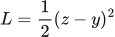 LaTeX:
L=\frac12(z-y)^2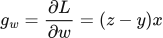 LaTeX:
g_w=\frac{\partial L}{\partial w}=(z-y)x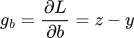 LaTeX:
g_b=\frac{\partial L}{\partial b}=z-y LaTeX:
w_{\mathrm{new}}=w-\eta g_w LaTeX:
b_{\mathrm{new}}=b-\eta g_bYaad rakhne ka cue: Ek path mein multiply; alag paths mil rahe hon toh add.
Solution — step by step
Meaning and formulas
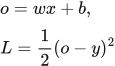
The output o is a linear prediction: no sigmoid or ReLU is specified. Changing w changes o, which changes L. The chain rule multiplies those linked effects.
 LaTeX:
o=wx+b,\qquad L=\frac12(o-y)^2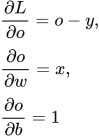 LaTeX:
\frac{\partial L}{\partial o}=o-y,\quad \frac{\partial o}{\partial w}=x,\quad \frac{\partial o}{\partial b}=1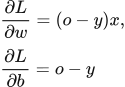 LaTeX:
\frac{\partial L}{\partial w}=(o-y)x,\qquad \frac{\partial L}{\partial b}=o-yThe learning rate η says how much of the gradient to subtract.
 LaTeX:
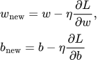
w_{\mathrm{new}}=w-\eta\frac{\partial L}{\partial w},\qquad b_{\mathrm{new}}=b-\eta\frac{\partial L}{\partial b}Step 1: obtain the current prediction and error
 LaTeX:
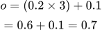
o=(0.2\times3)+0.1=0.6+0.1=0.7 LaTeX:
o-y=0.7-1=-0.3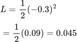 LaTeX:
L=\frac12(-0.3)^2=\frac12(0.09)=0.045Step 2: calculate both gradients from this same prediction
 LaTeX:
\frac{\partial L}{\partial w}=(-0.3)\times3=-0.9 LaTeX:
\frac{\partial L}{\partial b}=(-0.3)\times1=-0.3Step 3: update the weight
 LaTeX:
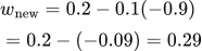
w_{\mathrm{new}}=0.2-0.1(-0.9)=0.2-(-0.09)=0.29Step 4: update the bias
 LaTeX:
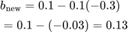
b_{\mathrm{new}}=0.1-0.1(-0.3)=0.1-(-0.03)=0.13Final answer: weight gradient −0.9; bias gradient −0.3; new weight 0.29; new bias 0.13. Both updates use the old forward pass.