Deep Learning · MT2 · section
All formulas: meanings, use and substitution
Formula reference and exam revision
These are the formulas used by this course. Each entry names its symbols and the type of calculation it serves. Numerical practice in the teaching chapters shows the longer working. Follow any different convention explicitly stated in the examination.
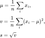
Formula 1: Mean, variance and standard deviation
 LaTeX:
\mu=\frac{1}{n}\sum_i x_i,\quad v=\frac{1}{n}\sum_i(x_i-\mu)^2,\quad s=\sqrt{v}Symbols: n is the count; mu is the mean; v is the population variance; s is the standard deviation.
Use: Use when calculating a population mean/variance or standardization. Sample-variance estimates may use n−1 when explicitly requested.
Substitution example: For [2,4]: mean = 3; deviations = −1,1; squares = 1,1; variance = 1; standard deviation = 1.
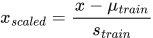
Formula 2: Standardization
 LaTeX:
x_{scaled}=\frac{x-\mu_{train}}{s_{train}}Symbols: Use the mean and standard deviation estimated from training data.
Use: Use to express a value relative to the training distribution. The standard deviation must be nonzero.
Substitution example: For x = 7, mean = 5, standard deviation = 2: (7−5)/2 = 1.
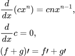
Formula 3: Power, constant and sum derivatives
 LaTeX:
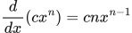
\frac{d}{dx}(cx^n)=cnx^{n-1},\quad\frac{d}{dx}c=0,\quad (f+g)\prime=f\prime+g\primeSymbols: c is a constant, x is the changing variable and n is the power.
Use: Use to differentiate the loss supplied in a gradient-descent question.
Substitution example: For 0.7x³: derivative = 0.7 × 3 × x² = 2.1x².
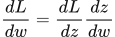
Formula 4: Chain rule
 LaTeX:
\frac{dL}{dw}=\frac{dL}{dz}\frac{dz}{dw}Symbols: z is the intermediate value linking w to L.
Use: Multiply derivatives along a path; add contributions from distinct paths that meet.
Substitution example: For z = 3w+1 and L = z² at w = 1: z = 4; derivative = (2×4)×3 = 24.
Formula 5: Dot product and a neuron
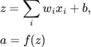 LaTeX:
z=\sum_i w_i x_i+b,\qquad a=f(z)Symbols: x is the input; w is its matching weight; b is one bias; z is the weighted sum; a is the activated output.
Use: Multiply each matching pair, add the products, add bias once, then activate.
Substitution example: x = [2,1], w = [0.5,−0.2], b = 0.1: z = 1−0.2+0.1 = 0.9.
Formula 6: Matrix multiplication
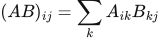 LaTeX:
(AB)_{ij}=\sum_k A_{ik}B_{kj}Symbols: i selects a row of A; j selects a column of B; k runs along the matching entries.
Use: Use row-times-column sums. A with shape m×n and B with n×p produces m×p.
Substitution example: Row [1,2] times column [3,4] gives 1×3+2×4 = 11.
Formula 7: Layer forward pass
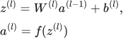 LaTeX:
z^{(l)}=W^{(l)}a^{(l-1)}+b^{(l)},\qquad a^{(l)}=f(z^{(l)})Symbols: l labels the layer; the previous layer activations become inputs to the next layer.
Use: For receiving-neuron rows, compute each row dot product and add that receiving neuron’s bias. Finish the whole layer before moving on.
Formula 8: Sigmoid and its derivative
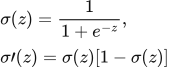 LaTeX:
\sigma(z)=\frac{1}{1+e^{-z}},\quad \sigma\prime(z)=\sigma(z)[1-\sigma(z)]Symbols: e is approximately 2.71828; sigma is the output.
Use: Use for a sigmoid forward pass and for its local backpropagation derivative.
Substitution example: At z = 0: output = 1/(1+1) = 0.5; derivative = 0.5×0.5 = 0.25.
Formula 9: Tanh and its derivative
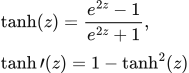 LaTeX:
\tanh(z)=\frac{e^{2z}-1}{e^{2z}+1},\quad \tanh\prime(z)=1-\tanh^2(z)Symbols: Tanh gives an output between −1 and 1.
Use: Use for a stated tanh activation, commonly an RNN hidden state or recurrent candidate.
Substitution example: At z = 0: numerator = 0, denominator = 2; output = 0; derivative = 1.
Formula 10: ReLU and its derivative
 LaTeX:
f(z)=\max(0,z),\quad f\prime(z)=\begin{cases}1&z>0\\0&z<0\end{cases}Symbols: max means choose the larger value.
Use: Use for ReLU. At zero the derivative is mathematically undefined; use the convention stated by the question or implementation.
Substitution example: For −2, output = 0 and derivative = 0. For 3, output = 3 and derivative = 1.
Formula 11: Leaky ReLU
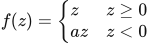 LaTeX:
f(z)=\begin{cases}z&z\geq0\\az&z<0\end{cases}Symbols: a is the small negative-side slope, commonly 0.01 unless specified.
Use: For negative z multiply by a; the output remains negative.
Substitution example: For z = −2 and a = 0.01: output = −0.02; derivative on this side is 0.01.
Formula 12: Stable softmax
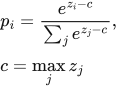 LaTeX:
p_i=\frac{e^{z_i-c}}{\sum_j e^{z_j-c}},\qquad c=\max_j z_jSymbols: z values are class scores; p values are probabilities.
Use: Subtract the same maximum from every score, exponentiate, add, divide each by that total.
Substitution example: For [0,0]: exponentials = [1,1]; total = 2; probabilities = [0.5,0.5].
Formula 13: Squared and absolute losses
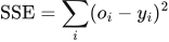 LaTeX:
\mathrm{SSE}=\sum_i(o_i-y_i)^2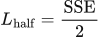 LaTeX:
L_{\mathrm{half}}=\frac{\mathrm{SSE}}2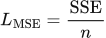 LaTeX:
L_{\mathrm{MSE}}=\frac{\mathrm{SSE}}n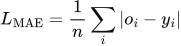 LaTeX:
L_{\mathrm{MAE}}=\frac1n\sum_i|o_i-y_i|Symbols: o is prediction; y is target; n is the number of averaged terms.
Use: Read whether the question uses a half sum, a mean, or an unhalved sum. The scaling changes gradients.
Substitution example: For errors [−1,2]: half sum = (1+4)/2 = 2.5; MSE = 2.5; MAE = (1+2)/2 = 1.5. The first two coincide only because n = 2.
Formula 14: Binary cross entropy
 LaTeX:
L=-[y\ln p+(1-y)\ln(1-p)]Symbols: y is 0 or 1; p is the predicted probability for class 1; ln is the natural logarithm.
Use: Use for a sigmoid binary prediction. If y = 1 use −ln(p); if y = 0 use −ln(1−p).
Substitution example: For y = 1 and p = 0.8: loss = 0.223144.
Formula 15: Categorical cross entropy
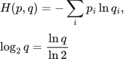 LaTeX:
H(p,q)=-\sum_i p_i\ln q_i,\qquad\log_2q=\frac{\ln q}{\ln2}For a soft target distribution, retain every nonzero target-weighted term. Natural logs give nats; base-2 logs give bits.
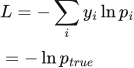 LaTeX:
L=-\sum_i y_i\ln p_i=-\ln p_{true}Symbols: The final equality assumes one-hot labels, with exactly one y equal to 1.
Use: Use for mutually exclusive multiclass labels. Select the probability of the true class.
Substitution example: True class 2 and probabilities [0.1,0.8,0.1]: loss = −ln(0.8) = 0.223144.
Formula 16: Output delta for half squared loss
 LaTeX:
\delta^{out}=(o-y)f\prime(z)Symbols: Delta is the loss derivative with respect to the preactivation z.
Use: Use with half squared loss. For unhalved one-output MSE multiply by 2; for an MSE averaged over m outputs multiply the half-sum delta by 2/m.
Substitution example: Sigmoid output 0.5 and target 1: delta = (−0.5)×0.25 = −0.125.
Formula 17: Sigmoid plus BCE; softmax plus CCE
 LaTeX:
\delta^{out}=p-ySymbols: p and y can be vectors for softmax.
Use: This is the combined derivative with respect to the logits. Do not multiply by the activation derivative again.
Substitution example: Binary p = 0.8, y = 1: delta = −0.2.
Formula 18: Hidden delta, weight gradient and bias gradient
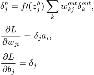 LaTeX:
\delta_j^h=f\prime(z_j^h)\sum_k w_{kj}^{out}\delta_k^{out},\quad\frac{\partial L}{\partial w_{ji}}=\delta_j a_i,\quad\frac{\partial L}{\partial b_j}=\delta_jSymbols: a_i is the activation sending a signal along the weight; delta_j belongs to the receiving neuron.
Use: Use OLD downstream weights throughout one backward pass. Add all outgoing-path contributions.
Substitution example: If receiving delta = −0.2 and sending activation = 3: weight gradient = −0.6; bias gradient = −0.2.
Formula 19: Gradient descent
 LaTeX:
\theta_{new}=\theta-\eta g,\qquad g=\frac{\partial J}{\partial\theta}Symbols: theta is the parameter; eta is learning rate; g is the current gradient.
Use: Recalculate g at the current parameter unless the question supplies gradients directly.
Substitution example: theta = 1, eta = 0.1, g = −2 gives 1−0.1(−2) = 1.2.
Formula 20: Batch and mini-batch gradient
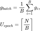 LaTeX:
g_{batch}=\frac1B\sum_{i=1}^{B}g_i,\quad U_{epoch}=\left\lceil\frac NB\right\rceilSymbols: B is batch size; N is sample count; U is updates per epoch when the final incomplete batch is retained.
Use: SGD uses B = 1. Full batch uses B = N. Average only when the stated objective is a mean.
Substitution example: N = 105, B = 20: six updates, with five samples in the last batch.
Formula 21: Momentum: signed velocity
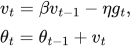 LaTeX:
v_t=\beta v_{t-1}-\eta g_t,\qquad\theta_t=\theta_{t-1}+v_tSymbols: v stores signed movement; beta retains part of old movement.
Use: Use this convention consistently. Other textbooks may define an unsigned gradient accumulator and subtract it instead.
Substitution example: beta = 0.8, old v = −0.2, eta = 0.1, g = 1.8 gives v = −0.34.
Formula 22: Nesterov: look-ahead gradient
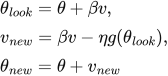 LaTeX:
\theta_{look}=\theta+\beta v,\quad v_{new}=\beta v-\eta g(\theta_{look}),\quad\theta_{new}=\theta+v_{new}Symbols: The look-ahead point is temporary; the update is added to the original theta.
Use: Evaluate the gradient at the look-ahead point, not at the old theta.
Substitution example: theta = 1.8, beta = 0.8 and v = −0.2 gives look-ahead = 1.64.
Formula 23: AdaGrad
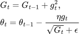 LaTeX:
G_t=G_{t-1}+g_t^2,\quad\theta_t=\theta_{t-1}-\frac{\eta g_t}{\sqrt{G_t}+\epsilon}Symbols: G is accumulated squared gradient; epsilon prevents division by zero.
Use: Accumulate every squared gradient, separately for each parameter. Use the epsilon placement stated by the problem.
Substitution example: Old G = 4 and g = −3 gives G = 13.
Formula 24: RMSProp
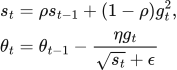 LaTeX:
s_t=\rho s_{t-1}+(1-\rho)g_t^2,\quad\theta_t=\theta_{t-1}-\frac{\eta g_t}{\sqrt{s_t}+\epsilon}Symbols: rho is the decay; s is a decaying mean of squared gradients.
Use: Calculate the new square memory first, then update the parameter.
Substitution example: rho = 0.9, old s = 4, g = −3 gives s = 3.6+0.9 = 4.5.
Formula 25: Adam: both memories
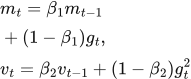 LaTeX:
m_t=\beta_1m_{t-1}+(1-\beta_1)g_t,\quad v_t=\beta_2v_{t-1}+(1-\beta_2)g_t^2Symbols: m remembers signed gradients; v remembers squared gradients.
Use: Start with the initial states specified. Common defaults are beta1 = 0.9 and beta2 = 0.999.
Formula 26: Adam: correction and update
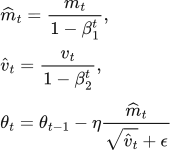 LaTeX:
\widehat m_t=\frac{m_t}{1-\beta_1^t},\quad\widehat v_t=\frac{v_t}{1-\beta_2^t},\quad\theta_t=\theta_{t-1}-\eta\frac{\widehat m_t}{\sqrt{\widehat v_t}+\epsilon}Symbols: t counts updates starting at 1, not 0.
Use: Correct both zero-initialized memories before the update; do not multiply by the gradient a second time.
Substitution example: At t = 1, m = 0.2 and beta1 = 0.9: corrected m = 0.2/0.1 = 2.
Formula 27: L1 penalty and update
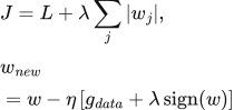 LaTeX:
J=L+\lambda\sum_j|w_j|,\quad w_{new}=w-\eta\left[g_{data}+\lambda\operatorname{sign}(w)\right]Symbols: lambda is regularization strength; sign(w) is +1 for positive w and −1 for negative w.
Use: At zero, L1 has a subgradient rather than a unique derivative; use the specified convention. Include only parameters named in the penalty.
Substitution example: w = −2, lambda = 0.1, data gradient = 0 gives penalty gradient = −0.1.
Formula 28: L2 penalty and update with a half
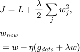 LaTeX:
J=L+\frac\lambda2\sum_jw_j^2,\quad w_{new}=w-\eta(g_{data}+\lambda w)Symbols: The half cancels the 2 produced by differentiating a square.
Use: If the objective uses lambda times the sum of squares WITHOUT a half, use 2 lambda w instead.
Substitution example: w = 2, lambda = 0.1, data gradient = 0.3 gives total gradient = 0.5.
Formula 29: Inverted dropout
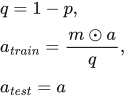 LaTeX:
q=1-p,\quad a_{train}=\frac{m\odot a}{q},\quad a_{test}=aSymbols: p is drop probability; q is keep probability; mask m contains zeros and ones; the circled dot means elementwise multiplication.
Use: During training, zero dropped entries and divide kept entries by q. Disable dropout at inference.
Substitution example: a = 3, q = 0.5, mask = 1 gives 3/0.5 = 6.
Formula 30: Convolution output dimensions
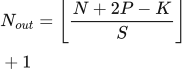 LaTeX:
N_{out}=\left\lfloor\frac{N+2P-K}{S}\right\rfloor+1Symbols: N is input height or width; P is padding on each side; K is kernel size; S is stride; floor rounds down.
Use: Apply separately to height and width. Output channels equal the number of filters. This formula assumes dilation 1.
Substitution example: N = 7, P = 1, K = 3, S = 2 gives floor(6/2)+1 = 4.
Formula 31: Convolution value
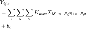 LaTeX:
Y_{ij,o}=\sum_c\sum_u\sum_v K_{uvco}X_{iS+u-P,jS+v-P,c}+b_oSymbols: c runs over input channels; u,v run over kernel positions; o selects one filter.
Use: This is the usual deep-learning cross-correlation operation. Use zeros outside the padded image. Multiply matching cells, add all channels, then add the filter bias once.
Formula 32: Max, min and average pooling
Min pooling keeps the smallest entry in each window. For a four-entry window:
 LaTeX:
y_{\min}=\min(x_1,x_2,x_3,x_4)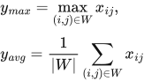 LaTeX:
y_{max}=\max_{(i,j)\in W}x_{ij},\quad y_{avg}=\frac1{|W|}\sum_{(i,j)\in W}x_{ij}Symbols: W is one pooling window; its size is the number of included cells.
Use: Move the window by the stated stride; process channels separately. For padding, follow the stated average-pooling denominator convention.
Substitution example: For [1,4,2,3]: maximum = 4; average = 10/4 = 2.5.
Formula 33: Convolution parameter count
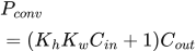 LaTeX:
P_{conv}=(K_hK_wC_{in}+1)C_{out}Symbols: Kernel height and width times input channels gives weights per filter; +1 is one bias; Cout is filter count.
Use: Use for a fully connected, ungrouped convolution with bias. Output height and width do not multiply the parameter count.
Substitution example: 3×3 kernel, 3 input channels, 2 filters: (27+1)×2 = 56.
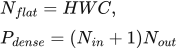
Formula 34: Flatten and dense parameter count
 LaTeX:
N_{flat}=HWC,\qquad P_{dense}=(N_{in}+1)N_{out}Symbols: H,W,C are activation dimensions; Nin and Nout are dense-layer input and output counts.
Use: Flatten has no trainable parameters. Dense biases belong to receiving neurons.
Substitution example: 2×2×2 flattens to 8; dense 3 then has (8+1)×3 = 27 parameters.
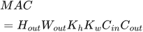
Formula 35: Convolution multiply-accumulate count
 LaTeX:
MAC=H_{out}W_{out}K_hK_wC_{in}C_{out}Symbols: Each output value uses kernel area times input-channel count multiplications.
Use: Used for Inception bottleneck comparisons. This counts one multiply-accumulate as one MAC and ignores bias additions. Some FLOP conventions count multiply and add separately.
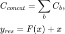
Formula 36: Concatenation and residual addition
 LaTeX:
C_{concat}=\sum_b C_b,\qquad y_{res}=F(x)+xSymbols: b labels branches with matching spatial dimensions.
Use: Inception concatenates channels; residual addition requires matching full shapes. Use a projection when needed.
Substitution example: Channels 16+32+8+8 give 64. Adding two 14×14×64 tensors keeps 14×14×64.
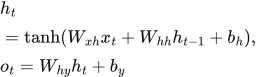
Formula 37: Vanilla RNN
 LaTeX:
h_t=\tanh(W_{xh}x_t+W_{hh}h_{t-1}+b_h),\quad o_t=W_{hy}h_t+b_ySymbols: x_t is current input; h_previous is previous state; the same matrices are reused at every time step.
Use: Calculate the two matrix-vector products, add bias, then tanh. Apply the stated output activation to o_t when required.
Formula 46: Batch normalization and learned scale/shift
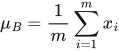
Use during training to normalize intermediate activations before a learned scale and shift. m is the number of values; μ_B and σ²_B are the batch mean and population variance; γ and β are learned. Epsilon is inside the square root. Ordinary inference uses stored running statistics. The linked full lesson calculates every stage for [2,4].
 LaTeX:
\mu_B=\frac{1}{m}\sum_{i=1}^{m}x_i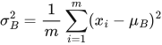 LaTeX:
\sigma_B^2=\frac{1}{m}\sum_{i=1}^{m}(x_i-\mu_B)^2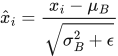 LaTeX:
\hat{x}_i=\frac{x_i-\mu_B}{\sqrt{\sigma_B^2+\epsilon}} LaTeX:
y_i=\gamma\hat{x}_i+\betaFormula 47: Global average pooling
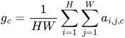
Take a separate average for each full spatial feature map. H and W count rows and columns; c selects one of C channels; a is an activation value. Output has C values. The linked lesson computes two channel averages and the following dense-layer parameters.
 LaTeX:
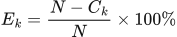
g_c=\frac{1}{HW}\sum_{i=1}^{H}\sum_{j=1}^{W}a_{i,j,c}Formula 48: Top-k error percentage
N is the total number of evaluated examples. C_k counts those whose true class is among the k highest-scoring predictions. Count failures, divide by total, then convert to percent. The worked lesson contrasts top-1 and top-5 using the same 100 images.
 LaTeX:
E_k=\frac{N-C_k}{N}\times100\%Expanded formula guide and worked examples
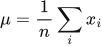
Mean, variance and standard deviation
The mean is a measure of location; variance and standard deviation quantify dispersion. Distinguish population and sample conventions before calculating these statistics.
 LaTeX:
\mu=\frac{1}{n}\sum_i x_i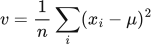 LaTeX:
v=\frac{1}{n}\sum_i(x_i-\mu)^2 LaTeX:
s=\sqrt{v}Mean, variance and standard deviation from ordinary arithmetic
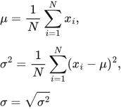
Definition. The arithmetic mean measures the centre of a numerical dataset. Variance measures the average squared deviation from that mean, and standard deviation expresses dispersion in the original units.
 LaTeX:
\mu=\frac{1}{N}\sum_{i=1}^{N}x_i,\qquad \sigma^2=\frac{1}{N}\sum_{i=1}^{N}(x_i-\mu)^2,\qquad \sigma=\sqrt{\sigma^2}These are population formulas, or empirical moments treating the supplied dataset as the complete reference set. An unbiased sample-variance estimate instead divides the squared-deviation sum by N−1. Use the convention specified by the question; the two denominators are not interchangeable.
Question. Find the population mean, variance and standard deviation of [3, 3, 7, 7].
Given
Observations = [3,3,7,7]; N = 4.
Use population variance (divide by N).
To find
Find the population mean μ, variance σ² and standard deviation σ.
Formula — which one and why
Mean and spread. The mean is the sum divided by the number of values. Population variance averages squared distances from that mean; standard deviation is its square root.
N = number of values; xᵢ = value i; μ = mean; σ² = variance; σ = standard deviation. Σ means add the indicated terms.
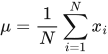 LaTeX:
\mu=\frac{1}{N}\sum_{i=1}^{N}x_i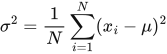 LaTeX:
\sigma^2=\frac{1}{N}\sum_{i=1}^{N}(x_i-\mu)^2 LaTeX:
\sigma=\sqrt{\sigma^2}Yaad rakhne ka cue: Mean = sabka total ÷ count; variance = squared distances ka mean.
Solution — step by step
Step 1: add all four observations.
 LaTeX:
3+3+7+7=20Step 2: divide by the count to obtain the mean.
 LaTeX:
\mu=\frac{20}{4}=5Step 3: subtract the mean from each observation.
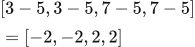 LaTeX:
[3-5,3-5,7-5,7-5]=[-2,-2,2,2]Step 4: square each deviation.
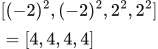 LaTeX:
[(-2)^2,(-2)^2,2^2,2^2]=[4,4,4,4]Step 5: add the squared deviations.
 LaTeX:
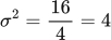
4+4+4+4=16Step 6: divide by four for population variance.
 LaTeX:
\sigma^2=\frac{16}{4}=4Step 7: take the nonnegative square root.
 LaTeX:
\sigma=\sqrt4=2Answer: mean = 5, population variance = 4 and population standard deviation = 2. Variance has squared units; standard deviation has the same units as the observations. With the sample convention, the variance would instead be 16/3.
Population mean and spread: [1, 2, 3]
Question. For the population [1, 2, 3], find mean, population variance and standard deviation.
Given
Values = [1, 2, 3]; N = 3. Use population division by N.
To find
Mean μ, variance σ² and standard deviation σ.
Formula — which one and why
The question specifies a population, so use N rather than the N−1 sample-variance divisor.
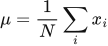
μ is the centre; σ² averages squared distances from it; σ converts spread back to the original units.
 LaTeX:
\mu=\frac1N\sum_i x_i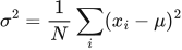 LaTeX:
\sigma^2=\frac1N\sum_i(x_i-\mu)^2LaTeX: \sigma=\sqrt{\sigma^2}Yaad rakhne ka cue: Mean, distance, square, mean again, then root.
Solution — step by step
Step 1: add all values.
 LaTeX:
1+2+3=6Step 2: divide by the number of values.
 LaTeX:
\mu=\frac{6}{3}=2Step 3: find and square deviation 1.
 LaTeX:
(1-2)=-1 LaTeX:
(-1)^2=1Step 4: find and square deviation 2.
 LaTeX:
(2-2)=0 LaTeX:
(0)^2=0Step 5: find and square deviation 3.
 LaTeX:
(3-2)=1 LaTeX:
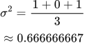
(1)^2=1Step 6: average the squared deviations.
 LaTeX:
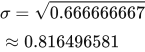
\sigma^2=\frac{1+0+1}{3}\approx0.666666667Step 7: take the nonnegative square root.
 LaTeX:
\sigma=\sqrt{0.666666667}\approx0.816496581Final answer: μ = 2; σ² ≈ 0.666666667; σ ≈ 0.816496581.
Population mean and spread: [2, 2, 2]
Question. For the population [2, 2, 2], find mean, population variance and standard deviation.
Given
Values = [2, 2, 2]; N = 3. Use population division by N.
To find
Mean μ, variance σ² and standard deviation σ.
Formula — which one and why
The question specifies a population, so use N rather than the N−1 sample-variance divisor.
μ is the centre; σ² averages squared distances from it; σ converts spread back to the original units.
LaTeX: \mu=\frac1N\sum_i x_iLaTeX: \sigma^2=\frac1N\sum_i(x_i-\mu)^2LaTeX: \sigma=\sqrt{\sigma^2}Yaad rakhne ka cue: Mean, distance, square, mean again, then root.
Solution — step by step
Step 1: add all values.
 LaTeX:
2+2+2=6Step 2: divide by the number of values.
LaTeX: \mu=\frac{6}{3}=2Step 3: find and square deviation 1.
LaTeX: (2-2)=0LaTeX: (0)^2=0Step 4: find and square deviation 2.
LaTeX: (2-2)=0LaTeX: (0)^2=0Step 5: find and square deviation 3.
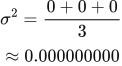
LaTeX: (2-2)=0LaTeX: (0)^2=0Step 6: average the squared deviations.
 LaTeX:
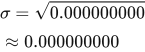
\sigma^2=\frac{0+0+0}{3}\approx0.000000000Step 7: take the nonnegative square root.
 LaTeX:
\sigma=\sqrt{0.000000000}\approx0.000000000Final answer: μ = 2; σ² ≈ 0.000000000; σ ≈ 0.000000000. Standardization is undefined with this zero standard deviation.
Standardization
Standardization has a meaning before it has a formula: measure how far an input is from its training mean, then express that distance in standard-deviation units. The worked question below calculates the mean and standard deviation first, so neither number appears without explanation.
LaTeX: x_{scaled}=\frac{x-\mu_{train}}{s_{train}}Standardization: what the answer 1 actually means
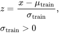
Definition. Standardization is an affine transformation that expresses an observation as its signed distance from a reference mean, measured in reference standard-deviation units.
 LaTeX:
z=\frac{x-\mu_{\mathrm{train}}}{\sigma_{\mathrm{train}}},\qquad \sigma_{\mathrm{train}}>0Subtracting the mean centres the reference data. Dividing by its standard deviation rescales its spread. The result is dimensionless. A positive z lies above the training mean, a negative z below it, and z = 0 equals it. Standardization does not make an arbitrary distribution Gaussian and does not restrict values to [0,1].
Question. A feature has training values [3, 3, 7, 7]. Using population standard deviation, standardize the training values and a new observation x = 9.
Given
Training observations = [3,3,7,7].
New observation = 9.
Estimate the population standard deviation from the training values.
To find
Find the training mean and standard deviation; standardize all four training values and the new observation.
Formula — which one and why
Mean and spread. The mean is the sum divided by the number of values. Population variance averages squared distances from that mean; standard deviation is its square root.
N = number of values; xᵢ = value i; μ = mean; σ² = variance; σ = standard deviation. Σ means add the indicated terms.
LaTeX: \mu=\frac{1}{N}\sum_{i=1}^{N}x_iLaTeX: \sigma^2=\frac{1}{N}\sum_{i=1}^{N}(x_i-\mu)^2LaTeX: \sigma=\sqrt{\sigma^2}Yaad rakhne ka cue: Mean = sabka total ÷ count; variance = squared distances ka mean.
Standardization. Subtract the training mean to measure distance from the centre; divide by the training standard deviation to express that distance in standard-deviation units.
x = original value; μ = training mean; σ = training standard deviation, which must be nonzero; z = standardized value.
 LaTeX:
z=\frac{x-\mu}{\sigma}Yaad rakhne ka cue: Pehle centre hatao, phir spread se divide karo.
Solution — step by step
Step 1: add all four observations.
LaTeX: 3+3+7+7=20Step 2: divide by the count to obtain the mean.
LaTeX: \mu=\frac{20}{4}=5Step 3: subtract the mean from each observation.
LaTeX: [3-5,3-5,7-5,7-5]=[-2,-2,2,2]Step 4: square each deviation.
LaTeX: [(-2)^2,(-2)^2,2^2,2^2]=[4,4,4,4]Step 5: add the squared deviations.
LaTeX: 4+4+4+4=16Step 6: divide by four for population variance.
LaTeX: \sigma^2=\frac{16}{4}=4Step 7: take the nonnegative square root.
LaTeX: \sigma=\sqrt4=2Step 8: standardize each original training observation.
 LaTeX:
\frac{3-5}{2}=-1 LaTeX:
\frac{7-5}{2}=1The repeated observations give [-1, −1, 1, 1].
Step 9: subtract the training mean from the new observation.
 LaTeX:
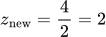
9-5=4Step 10: divide by the training standard deviation.
 LaTeX:
z_{\mathrm{new}}=\frac42=2Answer: the new observation is two training standard deviations above the training mean. Do not recompute the mean and standard deviation using the new observation; validation and test data use the training transformation to avoid leakage. A constant feature has zero standard deviation and needs a stated handling policy.
Standardization with x = 3
Question. Training mean is 5 and training standard deviation is 2. Standardize x = 3 and interpret the result.
Given
x = 3; training mean μ = 5; training standard deviation σ = 2.
To find
Standardized value z and its meaning.
Formula — which one and why
Subtract the training centre, then measure that distance in units of the training standard deviation.
A negative z means below the training mean; positive means above it; zero means equal to it.
LaTeX: z=\frac{x-\mu}{\sigma}Yaad rakhne ka cue: Centre hatao, spread se divide; answer batata hai kitne σ door.
Solution — step by step
Step 1: find distance from the mean.
 LaTeX:
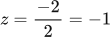
x-\mu=3-5=-2Step 2: divide by one standard-deviation unit.
 LaTeX:
z=\frac{-2}{2}=-1Step 3: interpret sign and size.
The value is 1 standard-deviation unit(s) below the training mean.
Final answer: z = -1. Use the same training statistics when transforming a new test input.
Standardization with x = 5
Question. Training mean is 5 and training standard deviation is 2. Standardize x = 5 and interpret the result.
Given
x = 5; training mean μ = 5; training standard deviation σ = 2.
To find
Standardized value z and its meaning.
Formula — which one and why
Subtract the training centre, then measure that distance in units of the training standard deviation.
A negative z means below the training mean; positive means above it; zero means equal to it.
LaTeX: z=\frac{x-\mu}{\sigma}Yaad rakhne ka cue: Centre hatao, spread se divide; answer batata hai kitne σ door.
Solution — step by step
Step 1: find distance from the mean.
 LaTeX:
x-\mu=5-5=0Step 2: divide by one standard-deviation unit.
 LaTeX:
z=\frac{0}{2}=0Step 3: interpret sign and size.
The value is 0 standard-deviation unit(s) away from the training mean.
Final answer: z = 0. Use the same training statistics when transforming a new test input.
Standardization with x = 9
Question. Training mean is 5 and training standard deviation is 2. Standardize x = 9 and interpret the result.
Given
x = 9; training mean μ = 5; training standard deviation σ = 2.
To find
Standardized value z and its meaning.
Formula — which one and why
Subtract the training centre, then measure that distance in units of the training standard deviation.
A negative z means below the training mean; positive means above it; zero means equal to it.
LaTeX: z=\frac{x-\mu}{\sigma}Yaad rakhne ka cue: Centre hatao, spread se divide; answer batata hai kitne σ door.
Solution — step by step
Step 1: find distance from the mean.
 LaTeX:
x-\mu=9-5=4Step 2: divide by one standard-deviation unit.
 LaTeX:
z=\frac{4}{2}=2Step 3: interpret sign and size.
The value is 2 standard-deviation unit(s) above the training mean.
Final answer: z = 2. Use the same training statistics when transforming a new test input.
Power, constant and sum derivatives
Derivatives describe local rates of change. Partial derivatives hold other independent variables fixed; their collection forms the gradient used for optimization.
 LaTeX:
\frac{d}{dx}(cx^n)=cnx^{n-1} LaTeX:
\frac{d}{dx}c=0 LaTeX:
(f+g)\prime=f\prime+g\primeDerivatives without a calculus course
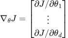
Definition. A derivative measures the local rate of change of a function. A partial derivative varies one argument while holding the others fixed. The gradient of a scalar-valued function collects its partial derivatives into a vector.
 LaTeX:
\nabla_\theta J=\begin{bmatrix}\partial J/\partial\theta_1\\\vdots\\\partial J/\partial\theta_d\end{bmatrix}The rules needed for the supplied neural-network numericals are:
| Function or operation | Derivative |
|---|---|
| Constant c | 0 |
| xⁿ | nxⁿ⁻¹ |
| c f(x) | c f′(x) |
| f(x) + g(x) | f′(x) + g′(x) |
| f(x)g(x) | f′(x)g(x) + f(x)g′(x) |
| eˣ | eˣ |
| ln x, x > 0 | 1/x |
| f(g(x)) | f′(g(x))g′(x) |
A parameter derivative is not an input derivative
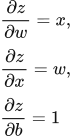
For z = wx + b, the variable named in the denominator determines which derivative is required.
 LaTeX:
\frac{\partial z}{\partial w}=x,\qquad\frac{\partial z}{\partial x}=w,\qquad\frac{\partial z}{\partial b}=1At x = 2, w = 3 and b = 1, z = 7, but the three derivatives are 2, 3 and 1 respectively. A function value and its derivative are distinct quantities.
Gradient direction
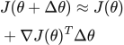
For a small parameter displacement Δθ, first-order Taylor expansion gives:
 LaTeX:
J(\theta+\Delta\theta)\approx J(\theta)+\nabla J(\theta)^T\Delta\thetaThe gradient points in the direction of greatest local increase under the Euclidean norm. Choosing Δθ opposite to the gradient gives a local descent direction. This is the mathematical basis of gradient descent; a finite step can still overshoot if the learning rate is too large.
Differentiate before substituting: 3w^2+5
Question. Let J(w) = 3w^2+5. At w = 2, find J and dJ/dw.
Given
J(w) = 3w^2+5; w = 2.
To find
The function value and its derivative value.
Formula — which one and why
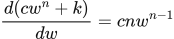
The power rule brings the exponent down as a multiplier and reduces its power by one. An added constant has derivative zero.
c is the coefficient; n is the power; k is an added constant. J and dJ/dw are different quantities.
 LaTeX:
\frac{d(cw^n+k)}{dw}=cnw^{n-1}Yaad rakhne ka cue: Power neeche multiply; exponent ek kam; constant ka zero.
Solution — step by step
Step 1: evaluate the function itself.
 LaTeX:
J(2)=3(2)^2+5=17Step 2: differentiate symbolically.
 LaTeX:
J\prime(w)=3(2)w^{2-1}+0Step 3: put the given w into the derivative.
 LaTeX:
J\prime(2)=3(2)(2)^{1}=12Final answer: J = 17; derivative = 12.
Differentiate before substituting: 0.7w^3+0
Question. Let J(w) = 0.7w^3+0. At w = 1, find J and dJ/dw.
Given
J(w) = 0.7w^3+0; w = 1.
To find
The function value and its derivative value.
Formula — which one and why
The power rule brings the exponent down as a multiplier and reduces its power by one. An added constant has derivative zero.
c is the coefficient; n is the power; k is an added constant. J and dJ/dw are different quantities.
LaTeX: \frac{d(cw^n+k)}{dw}=cnw^{n-1}Yaad rakhne ka cue: Power neeche multiply; exponent ek kam; constant ka zero.
Solution — step by step
Step 1: evaluate the function itself.
 LaTeX:
J(1)=0.7(1)^3+0=0.7Step 2: differentiate symbolically.
 LaTeX:
J\prime(w)=0.7(3)w^{3-1}+0Step 3: put the given w into the derivative.
 LaTeX:
J\prime(1)=0.7(3)(1)^{2}=2.1Final answer: J = 0.7; derivative = 2.1.
Differentiate before substituting: 2w^1+4
Question. Let J(w) = 2w^1+4. At w = -1, find J and dJ/dw.
Given
J(w) = 2w^1+4; w = -1.
To find
The function value and its derivative value.
Formula — which one and why
The power rule brings the exponent down as a multiplier and reduces its power by one. An added constant has derivative zero.
c is the coefficient; n is the power; k is an added constant. J and dJ/dw are different quantities.
LaTeX: \frac{d(cw^n+k)}{dw}=cnw^{n-1}Yaad rakhne ka cue: Power neeche multiply; exponent ek kam; constant ka zero.
Solution — step by step
Step 1: evaluate the function itself.
 LaTeX:
J(-1)=2(-1)^1+4=2Step 2: differentiate symbolically.
 LaTeX:
J\prime(w)=2(1)w^{1-1}+0Step 3: put the given w into the derivative.
 LaTeX:
J\prime(-1)=2(1)(-1)^{0}=2Final answer: J = 2; derivative = 2.
Chain rule
The chain rule differentiates a composite function. Multiply local derivatives along a dependency path and add the contributions of different paths to the same variable.
LaTeX: \frac{dL}{dw}=\frac{dL}{dz}\frac{dz}{dw}The chain rule is multiplying linked effects
Definition. The chain rule finds a rate of change when one quantity depends on another through intermediate calculations. Multiply the local rates along one path. If several paths connect the same starting quantity to the final answer, add their complete contributions.
First understand why the rates multiply
Suppose w controls u and u controls v. If each one-unit change in w makes u change by 3 units, and each one-unit change in u makes v change by 2 units, the combined rate is 3 × 2 = 6. Adding 3+2 would describe neither dependency.
The notation du/dw reads “the rate at which u changes when w changes”. A partial derivative ∂L/∂w means the same kind of rate while other independent parameters are held fixed. It is not ordinary division of the values L and w.
Yaad rakhne ka cue: ek raaste par slopes multiply; alag raaston ke full answers add.
Chain-rule example 1: two linear links
Question. Let u = 3w+1 and v = 2u. At w = 1, find u, v and dv/dw.
Given
w = 1; u = 3w+1; v = 2u.
To find
The two function values and the rate dv/dw.
Formula — which one and why
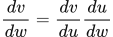
v depends on w through u. Both links must be included, so multiply the two local derivatives.
du/dw is the slope of 3w+1. dv/du is the slope of 2u.
 LaTeX:
\frac{dv}{dw}=\frac{dv}{du}\frac{du}{dw}Yaad rakhne ka cue: Andar ka slope × bahar ka slope.
Solution — step by step
Step 1: calculate the intermediate value.
 LaTeX:
u=3(1)+1=4Step 2: calculate the final value.
 LaTeX:
v=2(4)=8Step 3: differentiate the first link.
 LaTeX:
\frac{du}{dw}=3Step 4: differentiate the second link.
 LaTeX:
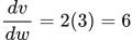
\frac{dv}{du}=2Step 5: multiply along the path.
 LaTeX:
\frac{dv}{dw}=2(3)=6Final answer: u = 4, v = 8 and dv/dw = 6. The function value 8 and its rate 6 are different.
2. One output: calculate both parameter gradients
Question. A linear neuron has z = wx + b and half squared loss L = ½(z − y)². Given x = 2, y = 4, w = 1 and b = 0, obtain both parameter gradients and perform one gradient-descent update with η = 0.1.
Given
Input x = 2; target y = 4.
Old weight w = 1; old bias b = 0.
Linear prediction z = wx+b; loss L = ½(z−y)².
Learning rate η = 0.1; update both parameters once.
To find
Find the loss gradient for w and for b, then w_new and b_new. Finally evaluate the changed prediction and loss.
Formula — which one and why
Chain rule for a linear neuron. The weight changes the prediction, and the prediction changes the loss. Multiply those two local rates. Half squared loss differentiates to prediction minus target; the neuron contributes input x.
z = prediction; y = target; e = z−y; g_w and g_b = loss derivatives for weight and bias. ∂L/∂w means “how fast loss changes when w changes”. η (eta) = learning rate.
 LaTeX:
z=wx+b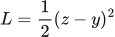 LaTeX:
L=\frac12(z-y)^2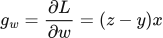 LaTeX:
g_w=\frac{\partial L}{\partial w}=(z-y)x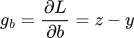 LaTeX:
g_b=\frac{\partial L}{\partial b}=z-y LaTeX:
w_{\mathrm{new}}=w-\eta g_w LaTeX:
b_{\mathrm{new}}=b-\eta g_bYaad rakhne ka cue: Ek path mein multiply; alag paths mil rahe hon toh add.
Solution — step by step
Step 1 — evaluate the original model. Use the given parameters before applying any update.
 LaTeX:
z=wx+b=1(2)+0=2 LaTeX:
e=z-y=2-4=-2 LaTeX:
L=\frac12e^2=\frac12(-2)^2=2The prediction is 2, the signed error is −2 and the loss is 2. These are three different quantities, even when some numerical values happen to coincide.
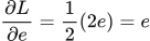
Step 2 — differentiate the loss, keeping the target constant. First differentiate the square, then the error inside it.
 LaTeX:
\frac{\partial L}{\partial e}=\frac12(2e)=e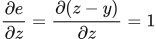 LaTeX:
\frac{\partial e}{\partial z}=\frac{\partial(z-y)}{\partial z}=1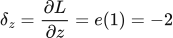 LaTeX:
\delta_z=\frac{\partial L}{\partial z}=e(1)=-2The symbol δ (delta) is a convenient name for the derivative with respect to a neuron's preactivation. Delta is not automatically the weight gradient; the weight gradient also depends on the input to that connection.
Step 3 — differentiate the neuron's affine expression. When differentiating with respect to w, x is a constant coefficient. When differentiating with respect to b, the coefficient of b is 1.
 LaTeX:
\frac{\partial z}{\partial w}=x=2 LaTeX:
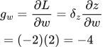
\frac{\partial z}{\partial b}=1Step 4 — multiply along each parameter's path.
 LaTeX:
g_w=\frac{\partial L}{\partial w}=\delta_z\frac{\partial z}{\partial w}=(-2)(2)=-4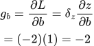 LaTeX:
g_b=\frac{\partial L}{\partial b}=\delta_z\frac{\partial z}{\partial b}=(-2)(1)=-2Both derivatives use the original forward-pass values. The weight and bias are different parameters, so keep their gradients separate.
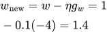
Step 5 — update both parameters simultaneously. Gradient descent subtracts the learning rate times the corresponding gradient.
 LaTeX:
w_{\mathrm{new}}=w-\eta g_w=1-0.1(-4)=1.4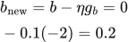 LaTeX:
b_{\mathrm{new}}=b-\eta g_b=0-0.1(-2)=0.2Both updates use gradients from the same original forward pass. Re-evaluate the model afterward.
Subtracting a negative gradient increases the parameter. Do not recompute the bias gradient using the already changed weight; that would be a different update procedure.
Step 6 — perform a new forward pass to evaluate the update.
 LaTeX:
z_{\mathrm{new}}=1.4(2)+0.2=3 LaTeX:
L_{\mathrm{new}}=\frac12(3-4)^2=0.5Final answer: weight gradient −4, bias gradient −2; updated weight 1.4 and bias 0.2; new prediction 3 and loss 0.5. If a different question fixes the bias at zero, update only the weight; its new prediction would be 2.8, not 3.
3. Two outputs: why backward contributions are added
A shared intermediate value can influence more than one output. The derivative with respect to that shared value must include every output path. Adding paths happens before passing the accumulated derivative further backward.
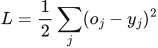
Question. A shared linear hidden value is h = wx + b. Two linear outputs are o₁ = 2h and o₂ = −h; their targets are y₁ = 1 and y₂ = 0. The total loss is L = ½(o₁ − y₁)² + ½(o₂ − y₂)². At x = 2, w = 0.5 and b = 0.1, calculate the loss and the gradients with respect to h, w and b. Treat the output multipliers 2 and −1 as fixed.
Given
h = wx+b; outputs o₁ = 2h and o₂ = −h.
x = 2; w = 0.5; b = 0.1; targets = [1,0].
Loss = half the sum of the two squared output errors.
Output multipliers 2 and −1 stay fixed.
To find
Find total loss and its derivatives with respect to h, w and b.
Formula — which one and why
Chain rule with more than one path. The shared hidden value affects each output. Multiply derivatives within each path, then add the complete path contributions before continuing to w and b.
oⱼ = output j; yⱼ = its target; h = shared hidden value; ∂oⱼ/∂h is the multiplier on that output path.
 LaTeX:
L=\frac12\sum_j(o_j-y_j)^2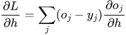 LaTeX:
\frac{\partial L}{\partial h}=\sum_j(o_j-y_j)\frac{\partial o_j}{\partial h} LaTeX:
\frac{\partial L}{\partial w}=\frac{\partial L}{\partial h}x LaTeX:
\frac{\partial L}{\partial b}=\frac{\partial L}{\partial h}Yaad rakhne ka cue: Har raaste ka effect pehle multiply, junction par sab add.
Solution — step by step
Step 1 — forward values.
 LaTeX:
h=0.5(2)+0.1=1.1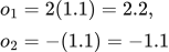 LaTeX:
o_1=2(1.1)=2.2,\qquad o_2=-(1.1)=-1.1 LaTeX:
L_1=\frac12(2.2-1)^2=0.72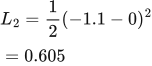 LaTeX:
L_2=\frac12(-1.1-0)^2=0.605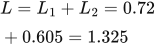 LaTeX:
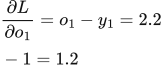
L=L_1+L_2=0.72+0.605=1.325Step 2 — output derivatives. Each half squared loss differentiates to prediction minus target. The other loss does not depend on this output.
 LaTeX:
\frac{\partial L}{\partial o_1}=o_1-y_1=2.2-1=1.2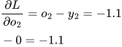 LaTeX:
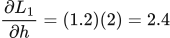
\frac{\partial L}{\partial o_2}=o_2-y_2=-1.1-0=-1.1Step 3 — calculate the contribution of each complete path. The derivative of 2h with respect to h is 2; the derivative of −h is −1.
 LaTeX:
\frac{\partial L_1}{\partial h}=(1.2)(2)=2.4 LaTeX:
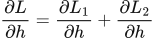
\frac{\partial L_2}{\partial h}=(-1.1)(-1)=1.1Step 4 — add the two contributions at the shared hidden value.
 LaTeX:
\frac{\partial L}{\partial h}=\frac{\partial L_1}{\partial h}+\frac{\partial L_2}{\partial h}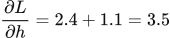 LaTeX:
\frac{\partial L}{\partial h}=2.4+1.1=3.5Adding the raw output errors, 1.2 + (−1.1), would omit the output multipliers. Each error must first be multiplied by the local derivative on its own path.
Step 5 — continue to the hidden weight and bias. Since h = wx + b, its derivatives with respect to w and b are x and 1.
 LaTeX:
\frac{\partial L}{\partial w}=\frac{\partial L}{\partial h}x=3.5(2)=7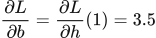 LaTeX:
\frac{\partial L}{\partial b}=\frac{\partial L}{\partial h}(1)=3.5Final answer: L = 1.325, ∂L/∂h = 3.5, ∂L/∂w = 7 and ∂L/∂b = 3.5. If the hidden value instead includes a nonlinear activation, multiply the accumulated downstream derivative by that activation's derivative before multiplying by x. This is the hidden-delta calculation in multilayer backpropagation.
Chain-rule example 4: a square after a linear link
Question. Let z = 3w+1 and L = z². At w = 1, find z, L and dL/dw.
Given
w = 1; z = 3w+1; L = z².
To find
z, L and the derivative of L with respect to w.
Formula — which one and why
The square acts on z, not directly on w. Differentiate the square first and include the change of z with w.
dL/dz = slope of the outer square; dz/dw = slope of the inner linear expression.
LaTeX: \frac{dL}{dw}=\frac{dL}{dz}\frac{dz}{dw} LaTeX:
\frac{d(z^2)}{dz}=2zYaad rakhne ka cue: Square ka 2z; andar ka 3; dono multiply.
Solution — step by step
Step 1: evaluate the inner expression.
 LaTeX:
z=3(1)+1=4Step 2: evaluate the loss expression.
 LaTeX:
L=4^2=16Step 3: differentiate the square and use z = 4.
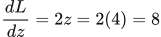 LaTeX:
\frac{dL}{dz}=2z=2(4)=8Step 4: differentiate the inner expression.
 LaTeX:
\frac{dz}{dw}=3Step 5: multiply, because the changes occur in sequence.
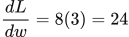 LaTeX:
\frac{dL}{dw}=8(3)=24Final answer: z = 4, L = 16 and dL/dw = 24. The combined operation is multiplication, not 8+3.
Drill 6 Chain rule on a tiny loss
Question
Question. Let o = wx+b, L = ½(o−y)², x = 3, w = 0.2, b = 0.1, y = 1. Find dL/dw, dL/db and update at η = 0.1.
Answer — step by step
Given
Model: o = wx+b; loss L = ½(o−y)².
x = 3; y = 1; w = 0.2; b = 0.1.
Learning rate η = 0.1.
To find
Find ∂L/∂w, ∂L/∂b and the updated weight and bias.
Formula — which one and why
Chain rule for a linear neuron. The weight changes the prediction, and the prediction changes the loss. Multiply those two local rates. Half squared loss differentiates to prediction minus target; the neuron contributes input x.
z = prediction; y = target; e = z−y; g_w and g_b = loss derivatives for weight and bias. ∂L/∂w means “how fast loss changes when w changes”. η (eta) = learning rate.
LaTeX: z=wx+bLaTeX: L=\frac12(z-y)^2LaTeX: g_w=\frac{\partial L}{\partial w}=(z-y)xLaTeX: g_b=\frac{\partial L}{\partial b}=z-yLaTeX: w_{\mathrm{new}}=w-\eta g_wLaTeX: b_{\mathrm{new}}=b-\eta g_bYaad rakhne ka cue: Ek path mein multiply; alag paths mil rahe hon toh add.
Solution — step by step
Meaning and formulas
The output o is a linear prediction: no sigmoid or ReLU is specified. Changing w changes o, which changes L. The chain rule multiplies those linked effects.
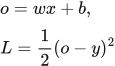 LaTeX:
o=wx+b,\qquad L=\frac12(o-y)^2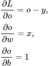 LaTeX:
\frac{\partial L}{\partial o}=o-y,\quad \frac{\partial o}{\partial w}=x,\quad \frac{\partial o}{\partial b}=1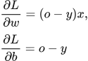 LaTeX:
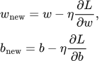
\frac{\partial L}{\partial w}=(o-y)x,\qquad \frac{\partial L}{\partial b}=o-yThe learning rate η says how much of the gradient to subtract.
 LaTeX:
w_{\mathrm{new}}=w-\eta\frac{\partial L}{\partial w},\qquad b_{\mathrm{new}}=b-\eta\frac{\partial L}{\partial b}Step 1: obtain the current prediction and error
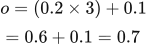 LaTeX:
o=(0.2\times3)+0.1=0.6+0.1=0.7 LaTeX:
o-y=0.7-1=-0.3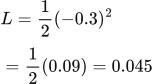 LaTeX:
L=\frac12(-0.3)^2=\frac12(0.09)=0.045Step 2: calculate both gradients from this same prediction
 LaTeX:
\frac{\partial L}{\partial w}=(-0.3)\times3=-0.9 LaTeX:
\frac{\partial L}{\partial b}=(-0.3)\times1=-0.3Step 3: update the weight
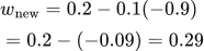 LaTeX:
w_{\mathrm{new}}=0.2-0.1(-0.9)=0.2-(-0.09)=0.29Step 4: update the bias
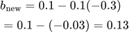 LaTeX:
b_{\mathrm{new}}=0.1-0.1(-0.3)=0.1-(-0.03)=0.13Final answer: weight gradient −0.9; bias gradient −0.3; new weight 0.29; new bias 0.13. Both updates use the old forward pass.
Dot product and a neuron
A neuron starts with matched input–weight pairs. Multiply inside each pair, add the products, add the bias once, and then apply the activation. The summation sign is simply a shorter way to write those additions.
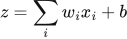 LaTeX:
z=\sum_i w_i x_i+b LaTeX:
a=f(z)Model answer: explain an artificial neuron
Question
Question. Explain the structure and working of an artificial neuron. Describe the roles of inputs, weights, bias and activation with a numerical example.
Answer — step by step
An artificial neuron is a computational unit that applies an activation function to an affine combination of its inputs. Its trainable weights and bias determine the preactivation; its output is passed to subsequent layers.
Formula and symbols
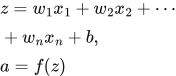 LaTeX:
z=w_1x_1+w_2x_2+\cdots+w_nx_n+b,\qquad a=f(z)| Part | Meaning | What it does |
|---|---|---|
| x₁, x₂, … | Input features | Supply the information for this calculation |
| w₁, w₂, … | Weights | Control the contribution of each matching input |
| b | Bias | Shifts the weighted sum independently of the inputs |
| z | Net input | The number before activation |
| f | Activation rule | Transforms z, often nonlinearly |
| a | Activated output | The number sent onward |
Worked ReLU neuron example
Question. An artificial neuron has x₁ = 2, x₂ = 1, w₁ = 0.5, w₂ = −0.2 and b = 0.1. Calculate its preactivation and ReLU output.
Given
Inputs = [2,1]; weights = [0.5,−0.2]; bias = 0.1; activation = ReLU.
To find
Preactivation z and activated output a.
Formula — which one and why
Each input contributes through its own weight. Add one bias after summing the products; ReLU then keeps a positive total.
z means before activation; a means after activation.
 LaTeX:
z=w_1x_1+w_2x_2+b LaTeX:
a=\max(0,z)Yaad rakhne ka cue: Product, product, sum, bias, phir activation.
Solution — step by step
Step 1: multiply the first pair.
 LaTeX:
0.5(2)=1Step 2: multiply the second pair.
 LaTeX:
(-0.2)(1)=-0.2Step 3: add both contributions.
 LaTeX:
1+(-0.2)=0.8Step 4: add the bias once.
 LaTeX:
z=0.8+0.1=0.9Step 5: apply ReLU.
 LaTeX:
a=\max(0,0.9)=0.9Final answer: z = 0.9 and a = 0.9. ReLU leaves this positive preactivation unchanged.
The weights and bias are learned parameters. During training, their values are adjusted to reduce an objective. The activation function itself is usually chosen as part of the architecture. Adding a bias does not mean adding one bias after every input product; add the receiving neuron's bias once.
What one artificial neuron does
Definition. An artificial neuron is a calculation unit that multiplies each input by a matching weight, adds the products and a bias, and applies an activation function to produce its output.
What goes into a neuron?
An input is a number supplied to the calculation. With three inputs, x = [2,1,3] simply lists those three numbers in order. The matching weight list tells the neuron which multiplier to use for each input. A negative weight contributes a negative amount when its input is positive.
The bias is one extra adjustable number added to the total. The total before activation is called z or preactivation. The activation function is the final rule applied to z: for example, ReLU replaces a negative z with zero, while sigmoid turns z into a number between 0 and 1. The resulting output is called a or the activation.
Yaad rakhne ka cue: inputs × apne weights → products ka sum → ek bias → activation → output.
Mathematical model and notation
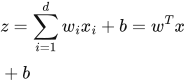 LaTeX:
z=\sum_{i=1}^{d}w_ix_i+b=w^Tx+bLaTeX: a=f(z)| Symbol | Meaning and role |
|---|---|
| xᵢ | Input component i; the neuron receives d such components |
| wᵢ | Trainable weight multiplying that input component |
| b | Trainable bias added once to this neuron's total |
| z | Preactivation: the result before applying the activation function |
| f | Chosen activation function, such as sigmoid or ReLU |
| a | Activation: the neuron's output after applying f |
The dot product wᵀx is a compact notation for the sum of matching weight–input products. A positive weight and a negative weight can make opposite contributions for the same positive input. A larger weight magnitude means a larger contribution for a fixed input; it is not, by itself, a general measure of feature importance across differently scaled inputs.
Why both a bias and an activation are needed
The bias changes the preactivation independently of x. In a one-input affine function z = wx + b, it is the intercept. In a classifier with a decision boundary z = 0, a bias allows that boundary to be shifted instead of forcing it through the origin.
The activation determines how z is transformed. Sigmoid produces a value between 0 and 1; ReLU retains positive preactivations and sets negative ones to zero. Nonlinear activations let stacked layers represent nonlinear functions. The preactivation and activation are distinct quantities even when a particular ReLU calculation gives them equal values.
Worked numerical
Question. A neuron has x = [2, 1, 3]ᵀ, w = [0.4, −0.2, 0.5]ᵀ and b = 0.1. Calculate its preactivation and sigmoid output.
Given
Inputs = [2,1,3]; matching weights = [0.4,−0.2,0.5].
Bias = 0.1; activation = sigmoid.
To find
Find the preactivation z, then the sigmoid output.
Formula — which one and why
Weighted sum and activation. Each input is multiplied by its connection weight. Add these contributions, add the bias once, then apply the stated activation.
xᵢ = input i; wᵢ = its weight; b = bias; z = sum before activation; a = output after activation; f = the specified activation function.
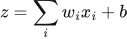 LaTeX:
z=\sum_iw_ix_i+bLaTeX: a=f(z)Yaad rakhne ka cue: Input × weight, sabka sum, bias once, phir activation.
Sigmoid output. The question specifies sigmoid, so turn the complete weighted sum into an output between 0 and 1. Negate z, evaluate the exponential, add 1, then take the reciprocal.
z = sum before activation; a = sigmoid output; e ≈ 2.71828 is the exponential base.
 LaTeX:
a=\frac1{1+e^{-z}}Yaad rakhne ka cue: Minus-z ki e power, plus one, phir one divided by whole denominator.
Solution — step by step
Step 1: multiply input 1 by weight 1.
 LaTeX:
x_1w_1=2(0.4)=0.8Step 2: multiply input 2 by weight 2.
 LaTeX:
x_2w_2=1(-0.2)=-0.2The minus sign belongs to the weight, so the contribution stays negative.
Step 3: multiply input 3 by weight 3.
 LaTeX:
x_3w_3=3(0.5)=1.5Step 4: add the three contributions.
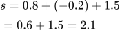 LaTeX:
s=0.8+(-0.2)+1.5=0.6+1.5=2.1Step 5: add the bias once.
 LaTeX:
z=s+b=2.1+0.1=2.2This is the preactivation. It is not yet the requested sigmoid output.
Step 6: negate z for the exponential.
 LaTeX:
-z=-2.2 LaTeX:
e^{-z}=e^{-2.2}\approx0.110803158Step 7: calculate the complete denominator.
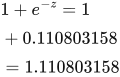 LaTeX:
1+e^{-z}=1+0.110803158=1.110803158Step 8: divide one by that denominator.
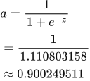 LaTeX:
a=\frac1{1+e^{-z}}=\frac1{1.110803158}\approx0.900249511Final answer: sigmoid output ≈ 0.900249511. It lies between 0 and 1. The raw sum was 2.2, whereas the activated output is approximately 0.90025.
From one neuron to a layer
With m receiving neurons and d input components, W has shape m × d. Row j contains the incoming weights of neuron j. The bias vector has m entries, one for each receiving neuron:
 LaTeX:
z=Wx+b,\qquad a=f(z)Sigmoid, tanh and ReLU apply independently to each component. Softmax is different: it transforms a whole vector of output logits together.
Neuron example 2: ReLU output
Question. A neuron receives inputs [2], weights [3] and bias 1. Calculate its preactivation and ReLU output.
Given
Inputs = [2].
Weights = [3]; bias = 1.
Activation = ReLU.
To find
z before activation and a after activation.
Formula — which one and why
The weighted sum combines the inputs. The output must then use the activation explicitly requested.
z names the sum; a names the activated result. They are not always equal.
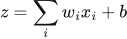 LaTeX:
z=\sum_i w_ix_i+bLaTeX: a=\max(0,z)Yaad rakhne ka cue: Sum alag, activation alag; activation lagana mat bhool.
Solution — step by step
Step 1: multiply input 1 by its own weight.
 LaTeX:
(2)(3)=6Step 2: add the input contributions.
 LaTeX:
s=(6)=6Step 3: add the bias once.
 LaTeX:
z=6+(1)=7Step 4: apply the stated activation.
 LaTeX:
a=\max(0,7)=7Final answer: z = 7; a = 7.
Neuron example 3: ReLU output
Question. A neuron receives inputs [2, 1], weights [-1, 0.5] and bias 0.2. Calculate its preactivation and ReLU output.
Given
Inputs = [2, 1].
Weights = [-1, 0.5]; bias = 0.2.
Activation = ReLU.
To find
z before activation and a after activation.
Formula — which one and why
The weighted sum combines the inputs. The output must then use the activation explicitly requested.
z names the sum; a names the activated result. They are not always equal.
LaTeX: z=\sum_i w_ix_i+bLaTeX: a=\max(0,z)Yaad rakhne ka cue: Sum alag, activation alag; activation lagana mat bhool.
Solution — step by step
Step 1: multiply input 1 by its own weight.
 LaTeX:
(2)(-1)=-2Step 2: multiply input 2 by its own weight.
 LaTeX:
(1)(0.5)=0.5Step 3: add the input contributions.
 LaTeX:
s=(-2)+(0.5)=-1.5Step 4: add the bias once.
 LaTeX:
z=-1.5+(0.2)=-1.3Step 5: apply the stated activation.
 LaTeX:
a=\max(0,-1.3)=0Final answer: z = -1.3; a = 0.
Neuron example 4: sigmoid output
Question. A neuron receives inputs [1, 2], weights [0.2, -0.1] and bias 0. Calculate its preactivation and sigmoid output.
Given
Inputs = [1, 2].
Weights = [0.2, -0.1]; bias = 0.
Activation = sigmoid.
To find
z before activation and a after activation.
Formula — which one and why
The weighted sum combines the inputs. The output must then use the activation explicitly requested.
z names the sum; a names the activated result. They are not always equal.
LaTeX: z=\sum_i w_ix_i+bLaTeX: a=\frac1{1+e^{-z}}Yaad rakhne ka cue: Sum alag, activation alag; activation lagana mat bhool.
Solution — step by step
Step 1: multiply input 1 by its own weight.
 LaTeX:
(1)(0.2)=0.2Step 2: multiply input 2 by its own weight.
 LaTeX:
(2)(-0.1)=-0.2Step 3: add the input contributions.
 LaTeX:
s=(0.2)+(-0.2)=0Step 4: add the bias once.
 LaTeX:
z=0+(0)=0Step 5: apply the stated activation.
 LaTeX:
a=\frac1{1+e^{0}}=\frac1{1+1}=0.5Final answer: z = 0; a = 0.5.
Drill 4 Dot product and bias
Question
Question. Find z for x = [2,−1,0.5], w = [0.3,0.4,−0.2], b = 0.1; then apply ReLU.
Answer — step by step
Given
Inputs x = [2, −1, 0.5].
Weights w = [0.3, 0.4, −0.2]; bias b = 0.1.
Activation: ReLU.
To find
Find the weighted sum z and ReLU output.
Formula — which one and why
Weighted sum and activation. Each input is multiplied by its connection weight. Add these contributions, add the bias once, then apply the stated activation.
xᵢ = input i; wᵢ = its weight; b = bias; z = sum before activation; a = output after activation; f = the specified activation function.
LaTeX: z=\sum_iw_ix_i+bLaTeX: a=f(z)Yaad rakhne ka cue: Input × weight, sabka sum, bias once, phir activation.
ReLU and Leaky ReLU. ReLU returns zero for negative input and retains positive input. Leaky ReLU instead multiplies a negative input by its supplied slope.
z = preactivation; α (alpha) = supplied negative-side slope for Leaky ReLU. The derivative at zero needs an explicit convention.
 LaTeX:
\operatorname{ReLU}(z)=\max(0,z) LaTeX:
\operatorname{LeakyReLU}(z)=\begin{cases}z&z\ge0\\\alpha z&z<0\end{cases}Yaad rakhne ka cue: Positive ko rehne do; negative ko zero. Leaky mein chhota negative rehne do.
Solution — step by step
Meaning and formulas
A dot product means multiply corresponding entries, then add the products. A bias is one extra value added after the sum. ReLU keeps a positive result and replaces a negative result with zero.
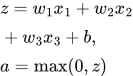 LaTeX:
z=w_1x_1+w_2x_2+w_3x_3+b,\qquad a=\max(0,z)Here x contains inputs, w contains weights, b is bias, z is the weighted sum, and a is the activated output.
Step 1: multiply the matching pairs
 LaTeX:
w_1x_1=0.3\times2=0.6 LaTeX:
w_2x_2=0.4\times(-1)=-0.4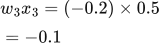 LaTeX:
w_3x_3=(-0.2)\times0.5=-0.1Step 2: add all products and add bias once
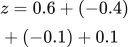 LaTeX:
z=0.6+(-0.4)+(-0.1)+0.1 LaTeX:
z=0.2-0.1+0.1=0.2Step 3: apply the activation
 LaTeX:
a=\max(0,0.2)=0.2Final answer: weighted sum z = 0.2; ReLU output a = 0.2. The two numbers happen to match because z is positive.
Matrix multiplication
Matrix multiplication implements affine transformations in a dense layer. Dimensions determine which products are valid; each output component is the dot product of a weight row and the input vector, plus its bias.
LaTeX: (AB)_{ij}=\sum_k A_{ik}B_{kj}Matrix multiplication: every row has a job
Row, column, vector and matrix — read these first
A row runs horizontally, from left to right. A column runs vertically, from top to bottom. A matrix is a rectangular arrangement of numbers in rows and columns. Its size is written rows × columns. A 2 × 3 matrix therefore has two rows and three columns, not six rows.
A vector is an ordered list of numbers. Written horizontally it is a row vector, such as [2, 1, 3]. Written vertically it is a column vector. Neural-network equations in these notes usually use column vectors.
Transpose: rows become columns
The superscript T means transpose, not a power. To obtain Aᵀ, copy row 1 of A as column 1, row 2 as column 2, and so on. Do not reverse the order within a row, change a sign or multiply anything. An m × n matrix becomes n × m.
 LaTeX:
[A^T]_{ij}=A_{ji}The two indices are positions: i identifies a row and j a column. The rule says “swap the row and column addresses”. For example, the value at row 1, column 3 moves to row 3, column 1.
Yaad rakhne ka cue: transpose = row ko column bana; number aur sign ko haath mat laga.
Transpose example 1
Question. Find the transpose of the following matrix A and state the size of both matrices.
Given
 LaTeX:
A=\begin{bmatrix}2&1&3\end{bmatrix}To find
Aᵀ and both matrix sizes.
Formula — which one and why
A transpose exchanges the row and column positions of every entry. It involves rearrangement, not multiplication.
A is the original matrix; Aᵀ is its transpose; i and j are row/column positions.
LaTeX: [A^T]_{ij}=A_{ji}Yaad rakhne ka cue: Row seedha column mein; double transpose se original wapas.
Solution — step by step
Step 1: write the original size.
A has 1 row(s) and 3 column(s), so its size is 1 × 3.
Step 2: move original row 1 into new column 1.
Copy [2, 1, 3] down column 1, in the same order.
Step 3: write the transposed matrix.
 LaTeX:
A^T=\begin{bmatrix}2\\1\\3\end{bmatrix}Step 4: state its new size.
The result has 3 row(s) and 1 column(s): 3 × 1.
Final answer: Aᵀ has size 3 × 1. Transposing it again gives the original A.
| 2 | 1 | 3 |
Read each colored row left to right.
| 2 |
| 1 |
| 3 |
Each original row is now the matching colored column.
The entry at row i, column j moves to row j, column i. Its value and sign do not change.
Transpose example 2
Question. Find the transpose of the following matrix A and state the size of both matrices.
Given
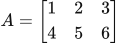 LaTeX:
A=\begin{bmatrix}1&2&3\\4&5&6\end{bmatrix}To find
Aᵀ and both matrix sizes.
Formula — which one and why
A transpose exchanges the row and column positions of every entry. It involves rearrangement, not multiplication.
A is the original matrix; Aᵀ is its transpose; i and j are row/column positions.
LaTeX: [A^T]_{ij}=A_{ji}Yaad rakhne ka cue: Row seedha column mein; double transpose se original wapas.
Solution — step by step
Step 1: write the original size.
A has 2 row(s) and 3 column(s), so its size is 2 × 3.
Step 2: move original row 1 into new column 1.
Copy [1, 2, 3] down column 1, in the same order.
Step 3: move original row 2 into new column 2.
Copy [4, 5, 6] down column 2, in the same order.
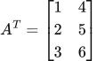
Step 4: write the transposed matrix.
 LaTeX:
A^T=\begin{bmatrix}1&4\\2&5\\3&6\end{bmatrix}Step 5: state its new size.
The result has 3 row(s) and 2 column(s): 3 × 2.
Final answer: Aᵀ has size 3 × 2. Transposing it again gives the original A.
| 1 | 2 | 3 |
| 4 | 5 | 6 |
Read each colored row left to right.
| 1 | 4 |
| 2 | 5 |
| 3 | 6 |
Each original row is now the matching colored column.
The entry at row i, column j moves to row j, column i. Its value and sign do not change.
Transpose example 3
Question. Find the transpose of the following matrix A and state the size of both matrices.
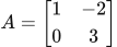
Given
 LaTeX:
A=\begin{bmatrix}1&-2\\0&3\end{bmatrix}To find
Aᵀ and both matrix sizes.
Formula — which one and why
A transpose exchanges the row and column positions of every entry. It involves rearrangement, not multiplication.
A is the original matrix; Aᵀ is its transpose; i and j are row/column positions.
LaTeX: [A^T]_{ij}=A_{ji}Yaad rakhne ka cue: Row seedha column mein; double transpose se original wapas.
Solution — step by step
Step 1: write the original size.
A has 2 row(s) and 2 column(s), so its size is 2 × 2.
Step 2: move original row 1 into new column 1.
Copy [1, -2] down column 1, in the same order.
Step 3: move original row 2 into new column 2.
Copy [0, 3] down column 2, in the same order.
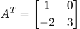
Step 4: write the transposed matrix.
 LaTeX:
A^T=\begin{bmatrix}1&0\\-2&3\end{bmatrix}Step 5: state its new size.
The result has 2 row(s) and 2 column(s): 2 × 2.
Final answer: Aᵀ has size 2 × 2. Transposing it again gives the original A.
| 1 | −2 |
| 0 | 3 |
Read each colored row left to right.
| 1 | 0 |
| −2 | 3 |
Each original row is now the matching colored column.
The entry at row i, column j moves to row j, column i. Its value and sign do not change.
Transpose example 4
Question. Find the transpose of the following matrix A and state the size of both matrices.
Given
 LaTeX:
A=\begin{bmatrix}-1\\4\\2\end{bmatrix}To find
Aᵀ and both matrix sizes.
Formula — which one and why
A transpose exchanges the row and column positions of every entry. It involves rearrangement, not multiplication.
A is the original matrix; Aᵀ is its transpose; i and j are row/column positions.
LaTeX: [A^T]_{ij}=A_{ji}Yaad rakhne ka cue: Row seedha column mein; double transpose se original wapas.
Solution — step by step
Step 1: write the original size.
A has 3 row(s) and 1 column(s), so its size is 3 × 1.
Step 2: move original row 1 into new column 1.
Copy [-1] down column 1, in the same order.
Step 3: move original row 2 into new column 2.
Copy [4] down column 2, in the same order.
Step 4: move original row 3 into new column 3.
Copy [2] down column 3, in the same order.
Step 5: write the transposed matrix.
 LaTeX:
A^T=\begin{bmatrix}-1&4&2\end{bmatrix}Step 6: state its new size.
The result has 1 row(s) and 3 column(s): 1 × 3.
Final answer: Aᵀ has size 1 × 3. Transposing it again gives the original A.
| −1 |
| 4 |
| 2 |
Read each colored row left to right.
| −1 | 4 | 2 |
Each original row is now the matching colored column.
The entry at row i, column j moves to row j, column i. Its value and sign do not change.
Dot product: multiply matching entries, then add
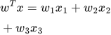
A dot product turns two equally long lists into one number. Match first with first, second with second, and so on. It is the weighted sum inside a neuron. If both lists are columns, wᵀ turns the weight column into a row so row × column is allowed.
 LaTeX:
w^Tx=w_1x_1+w_2x_2+w_3x_3This formula is the three-input case. With two inputs there are only two products; with d inputs there are d products. A bias is an additional term, added after these products.
Dot-product example 1
Question. For w = [2, 3] and x = [4, 1], calculate wᵀx.
Given
Weights w = [2, 3].
Matching inputs x = [4, 1].
Both lists contain 2 numbers.
To find
One scalar value wᵀx.
Formula — which one and why
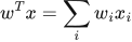
A dot product is a sum of matching products. There is no bias in this question.
Σ means add; the index i visits each matching pair.
 LaTeX:
w^Tx=\sum_i w_ix_iYaad rakhne ka cue: Same position multiply; sab products add.
Solution — step by step
Step 1: multiply matching pair 1.
 LaTeX:
(2)(4)=8Step 2: multiply matching pair 2.
 LaTeX:
(3)(1)=3Step 3: add the products.
 LaTeX:
w^Tx=(8)+(3)=11Final answer: wᵀx = 11.
Dot-product example 2
Question. For w = [1, -2] and x = [2, 3], calculate wᵀx.
Given
Weights w = [1, -2].
Matching inputs x = [2, 3].
Both lists contain 2 numbers.
To find
One scalar value wᵀx.
Formula — which one and why
A dot product is a sum of matching products. There is no bias in this question.
Σ means add; the index i visits each matching pair.
LaTeX: w^Tx=\sum_i w_ix_iYaad rakhne ka cue: Same position multiply; sab products add.
Solution — step by step
Step 1: multiply matching pair 1.
 LaTeX:
(1)(2)=2Step 2: multiply matching pair 2.
 LaTeX:
(-2)(3)=-6Step 3: add the products.
 LaTeX:
w^Tx=(2)+(-6)=-4Final answer: wᵀx = -4.
Dot-product example 3
Question. For w = [0.5, 1, -1] and x = [4, 2, 3], calculate wᵀx.
Given
Weights w = [0.5, 1, -1].
Matching inputs x = [4, 2, 3].
Both lists contain 3 numbers.
To find
One scalar value wᵀx.
Formula — which one and why
A dot product is a sum of matching products. There is no bias in this question.
Σ means add; the index i visits each matching pair.
LaTeX: w^Tx=\sum_i w_ix_iYaad rakhne ka cue: Same position multiply; sab products add.
Solution — step by step
Step 1: multiply matching pair 1.
 LaTeX:
(0.5)(4)=2Step 2: multiply matching pair 2.
LaTeX: (1)(2)=2Step 3: multiply matching pair 3.
 LaTeX:
(-1)(3)=-3Step 4: add the products.
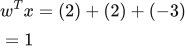 LaTeX:
w^Tx=(2)+(2)+(-3)=1Final answer: wᵀx = 1.
Matrix multiplication: each row makes one output
To multiply A of size m × n by B of size n × p, the inner sizes n must match. The result has size m × p. Output entry (i,j) is row i of A dotted with column j of B.
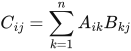 LaTeX:
C_{ij}=\sum_{k=1}^{n}A_{ik}B_{kj}For a layer receiving two inputs and producing two neuron outputs, W is 2 × 2, x is 2 × 1 and Wx is 2 × 1. Each row of W holds all weights entering one receiving neuron. Its matching bias is added once.
Yaad rakhne ka cue: multiplication mein andar ke sizes match; answer ka size bahar ke sizes. Har output = ek row × ek column.
Definition. A vector is an ordered collection of scalars; a matrix represents a linear transformation between vector spaces. A neural-network layer combines a linear transformation with an additive bias, giving an affine transformation.
 LaTeX:
z=Wx+bFor d input features and m receiving neurons, the dimensions are:
 LaTeX:
W\in\mathbb R^{m\times d},\quad x\in\mathbb R^{d\times1},\quad b,z\in\mathbb R^{m\times1}The inner dimensions must match. Output component j is the dot product of row j of W with x, plus bias bⱼ. Wᵀ reverses the matrix dimensions. The Hadamard product u⊙v multiplies corresponding components and is different from a matrix product.
Question. Given W =  LaTeX:
\begin{bmatrix}1 & -2\\0.5 & 3\end{bmatrix}, x = [2, 1]ᵀ and b = [0.1, −0.2]ᵀ, calculate z = Wx + b.
Given
Weights W = LaTeX: \begin{bmatrix}1 & -2\\0.5 & 3\end{bmatrix}.
Input column x = [2,1]ᵀ; bias column b = [0.1,−0.2]ᵀ.
To find
Find both components of z = Wx+b.
Formula — which one and why
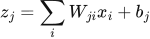
Row–column multiplication. Each receiving neuron uses one weight row. Multiply that row by the input column, add the products, then add that neuron’s bias.
Wⱼᵢ = weight from input i to receiver j; xᵢ = input i; bⱼ = bias of receiver j; zⱼ = its preactivation. A superscript T means transpose: exchange rows and columns.
 LaTeX:
z_j=\sum_i W_{ji}x_i+b_jYaad rakhne ka cue: Ek row × poora input column = ek receiving neuron ka answer.
Solution — step by step
Step 1: verify compatible dimensions.
W has 2 rows and 2 columns; x has 2 rows and 1 column. The inner dimensions match, and the result has 2 rows and 1 column.
Step 2: calculate the first receiving row products.
 LaTeX:
1(2)=2 LaTeX:
(-2)(1)=-2Step 3: sum row 1 and add its bias.
 LaTeX:
z_1=2+(-2)+0.1=0.1Step 4: calculate the second receiving row products.
LaTeX: 0.5(2)=1 LaTeX:
3(1)=3Step 5: sum row 2 and add its bias.
 LaTeX:
z_2=1+3-0.2=3.8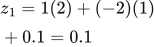 LaTeX:
z_1=1(2)+(-2)(1)+0.1=0.1| 1 | −2 |
| 0.5 | 3 |
| 2 |
| 1 |
| 2 | −2 |
First × first; second × second.
One receiving neuron corresponds to one row of W and one bias. The other weight row is not used for this component.
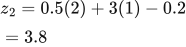 LaTeX:
z_2=0.5(2)+3(1)-0.2=3.8| 1 | −2 |
| 0.5 | 3 |
| 2 |
| 1 |
| 1 | 3 |
First × first; second × second.
One receiving neuron corresponds to one row of W and one bias. The other weight row is not used for this component.
 LaTeX:
z=\begin{bmatrix}0.1\\3.8\end{bmatrix}An activation is applied afterward if the question asks for the layer output. In backpropagation, the input gradient uses Wᵀ because it maps derivatives from m outputs back to d inputs. For a single example, an outer product δxᵀ produces a weight-gradient matrix with exactly the same dimensions as W.
Two output columns
Question. Multiply A =  LaTeX:
\begin{bmatrix}1 & 2\\3 & 4\end{bmatrix} by B =  LaTeX:
\begin{bmatrix}2 & 0\\1 & 3\end{bmatrix}. Show all four output entries.
Given
 LaTeX:
A=\begin{bmatrix}1&2\\3&4\end{bmatrix} LaTeX:
B=\begin{bmatrix}2&0\\1&3\end{bmatrix}To find
The 2 × 2 matrix C = AB.
Formula — which one and why
Matrix multiplication pairs one row of A with one column of B for each output. It is not entry-by-entry multiplication.
Cᵢⱼ is the entry in output row i, column j.
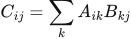 LaTeX:
C_{ij}=\sum_k A_{ik}B_{kj}Yaad rakhne ka cue: Output ki position dekho: wahi row, wahi column.
Solution — step by step
Step 1: check the dimensions.
(2 × 2)(2 × 2) is valid; output size = 2 × 2.
Step 2: row 1 with column 1.
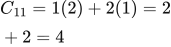 LaTeX:
C_{11}=1(2)+2(1)=2+2=4Step 3: row 1 with column 2.
 LaTeX:
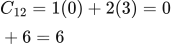
C_{12}=1(0)+2(3)=0+6=6Step 4: row 2 with column 1.
 LaTeX:
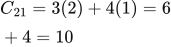
C_{21}=3(2)+4(1)=6+4=10Step 5: row 2 with column 2.
 LaTeX:
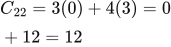
C_{22}=3(0)+4(3)=0+12=12Step 6: assemble the output by position.
 LaTeX:
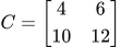
C=\begin{bmatrix}4&6\\10&12\end{bmatrix}Final answer: C =  LaTeX:
\begin{bmatrix}4 & 6\\10 & 12\end{bmatrix}, with size 2 × 2.
Two products that must not be confused
Question. Let a = [2,3]ᵀ and b = [4,5]ᵀ. Find the entry-by-entry product a ⊙ b and the outer product abᵀ.
Given
a and b are both 2 × 1 columns: a contains 2,3 and b contains 4,5.
To find
The 2 × 1 entry-by-entry product and the 2 × 2 outer product.
Formula — which one and why
⊙ multiplies corresponding positions; the outer product combines every value of a with every value of b. Backpropagation uses both operations for different reasons.
⊙ is called the Hadamard or elementwise product. bᵀ is a 1 × 2 row.
 LaTeX:
(a\odot b)_i=a_i b_i LaTeX:
(ab^T)_{ij}=a_i b_jYaad rakhne ka cue: ⊙ mein same jagah; outer product mein har pair.
Solution — step by step
Step 1: multiply matching entries.
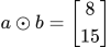 LaTeX:
a\odot b=\begin{bmatrix}8\\15\end{bmatrix}Step 2: transpose b.
 LaTeX:
b^T=\begin{bmatrix}4&5\end{bmatrix}Step 3: form row 1 of the outer product.
 LaTeX:
2(4)=8,\qquad2(5)=10Step 4: form row 2 of the outer product.
 LaTeX:
3(4)=12,\qquad3(5)=15Step 5: write both rows.
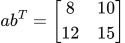 LaTeX:
ab^T=\begin{bmatrix}8&10\\12&15\end{bmatrix}Final answer: Entry-by-entry result = [8,15]ᵀ. Outer product =  LaTeX:
\begin{bmatrix}8 & 10\\12 & 15\end{bmatrix}.
Drill 5 Matrix rows receive inputs
Question
Question. For the weight matrix W shown below, x = [2,1], b = [0.5,−0.5], find Wx+b and ReLU.
Answer — step by step
Given
W =  LaTeX:
\begin{bmatrix}1 & 2\\-1 & 3\end{bmatrix}.
Input column x = [2,1]ᵀ; bias column b = [0.5,−0.5]ᵀ.
Activation: ReLU on each result.
To find
Find Wx+b and the activated output.
Formula — which one and why
Row–column multiplication. Each receiving neuron uses one weight row. Multiply that row by the input column, add the products, then add that neuron’s bias.
Wⱼᵢ = weight from input i to receiver j; xᵢ = input i; bⱼ = bias of receiver j; zⱼ = its preactivation. A superscript T means transpose: exchange rows and columns.
LaTeX: z_j=\sum_i W_{ji}x_i+b_jYaad rakhne ka cue: Ek row × poora input column = ek receiving neuron ka answer.
ReLU and Leaky ReLU. ReLU returns zero for negative input and retains positive input. Leaky ReLU instead multiplies a negative input by its supplied slope.
z = preactivation; α (alpha) = supplied negative-side slope for Leaky ReLU. The derivative at zero needs an explicit convention.
LaTeX: \operatorname{ReLU}(z)=\max(0,z)LaTeX: \operatorname{LeakyReLU}(z)=\begin{cases}z&z\ge0\\\alpha z&z<0\end{cases}Yaad rakhne ka cue: Positive ko rehne do; negative ko zero. Leaky mein chhota negative rehne do.
Solution — step by step
Meaning and formula
Each row supplies the weights of one receiving neuron. Multiply that row by the input column, then add that neuron's own bias. The two biases are separate; do not add both to every row.
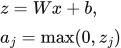 LaTeX:
z=Wx+b,\qquad a_j=\max(0,z_j) LaTeX:
W=\begin{bmatrix}1&2\\-1&3\end{bmatrix},\quad x=\begin{bmatrix}2\\1\end{bmatrix},\quad b=\begin{bmatrix}0.5\\-0.5\end{bmatrix}Step 1: calculate receiving neuron 1 from row 1
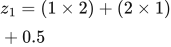 LaTeX:
z_1=(1\times2)+(2\times1)+0.5 LaTeX:
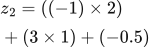
z_1=2+2+0.5=4.5Step 2: calculate receiving neuron 2 from row 2
 LaTeX:
z_2=((-1)\times2)+(3\times1)+(-0.5) LaTeX:
z_2=-2+3-0.5=0.5Step 3: apply ReLU to each entry
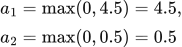 LaTeX:
a_1=\max(0,4.5)=4.5,\qquad a_2=\max(0,0.5)=0.5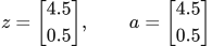 LaTeX:
z=\begin{bmatrix}4.5\\0.5\end{bmatrix},\qquad a=\begin{bmatrix}4.5\\0.5\end{bmatrix}The shape is 2 rows by 1 column: one output for each receiving row.
Layer forward pass
A layer does the neuron calculation for several receiving neurons. Finish all its outputs before using them as the next layer’s inputs. The bracketed superscript is a layer label, not a power.
 LaTeX:
z^{(l)}=W^{(l)}a^{(l-1)}+b^{(l)} LaTeX:
a^{(l)}=f(z^{(l)})Forward propagation through multiple neurons
Definitions. A feedforward neural network has a directed acyclic computation graph: information moves from inputs toward outputs without recurrent feedback connections. A multilayer perceptron (MLP) is a feedforward network built from fully connected layers, with one or more hidden layers and nonlinear hidden activations.
Input, hidden and output layers
The input layer supplies the feature vector. A hidden layer learns an intermediate representation; its outputs are computed from preceding activations, not supplied as target labels. The output layer produces the prediction in the form needed by the task.
In a dense connection between two layers, every receiving neuron has a weight for every preceding activation. Each receiving neuron also normally has its own bias. An ANN is the broader family containing feedforward and recurrent models. A CNN can be feedforward without being an MLP, because convolution uses local shared connections.
General layer equations and dimensions
Let a⁽⁰⁾ = x. For layer l:
LaTeX: z^{(l)}=W^{(l)}a^{(l-1)}+b^{(l)} LaTeX:
a^{(l)}=f^{(l)}(z^{(l)})If the preceding layer has n inputs and the current layer has m neurons, W has m rows and n columns. The vectors z, a and b have m components. Row j of W contains the incoming weights of neuron j.
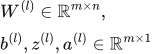 LaTeX:
W^{(l)}\in\mathbb R^{m\times n},\qquad b^{(l)},z^{(l)},a^{(l)}\in\mathbb R^{m\times1}For one hidden layer, these computations compose to give:
 LaTeX:
h=f^{(1)}(W^{(1)}x+b^{(1)}) LaTeX:
\hat y=f^{(2)}(W^{(2)}h+b^{(2)})The hidden activation must be nonlinear to obtain nonlinear representational power. Stacking affine layers alone still gives one affine mapping. A single threshold perceptron cannot separate XOR; a hidden nonlinear representation can make the two classes separable for the output layer.
Forward propagation versus training
Forward propagation evaluates these layer equations using the current parameters. Training additionally evaluates a loss, uses backpropagation to calculate gradients, and applies an optimizer update. The architecture specifies connections; backpropagation is a differentiation algorithm used to train that architecture.
Complete two-layer numerical
Question. A feedforward network receives x = [1, 0]ᵀ. Its hidden-layer weights are W¹ =  LaTeX:
\begin{bmatrix}0.2 & 0.4\\0.3 & 0.7\end{bmatrix} and biases are b¹ = [0.1, 0.2]ᵀ. The output weights are W² = [0.5, 0.6] and output bias is b² = 0.1. Use ReLU in both layers and one row per receiving neuron. Calculate every preactivation and the final output.
Given
A feedforward network receives x = [1, 0]ᵀ.
Its hidden-layer weights are W¹ = LaTeX: \begin{bmatrix}0.2 & 0.4\\0.3 & 0.7\end{bmatrix} and biases are b¹ = [0.1, 0.2]ᵀ.
The output weights are W² = [0.5, 0.6] and output bias is b² = 0.1.
Use ReLU in both layers and one row per receiving neuron.
To find
Find all preactivations, hidden activations and final outputs. Find the requested activation values and slopes.
Formula — which one and why
Forward propagation. Evaluate one layer completely before supplying its activated outputs to the next layer. Each layer has its own weights and biases.
x = input vector; h = hidden outputs; W₁,b₁ = hidden parameters; W₂,b₂ = output parameters; f₁,f₂ = the stated activations.
 LaTeX:
z_h=W_1x+b_1 LaTeX:
h=f_1(z_h) LaTeX:
z_o=W_2h+b_2 LaTeX:
o=f_2(z_o)Yaad rakhne ka cue: Pehli layer ka activated output hi agli layer ka input hai.
ReLU and Leaky ReLU. ReLU returns zero for negative input and retains positive input. Leaky ReLU instead multiplies a negative input by its supplied slope.
z = preactivation; α (alpha) = supplied negative-side slope for Leaky ReLU. The derivative at zero needs an explicit convention.
LaTeX: \operatorname{ReLU}(z)=\max(0,z)LaTeX: \operatorname{LeakyReLU}(z)=\begin{cases}z&z\ge0\\\alpha z&z<0\end{cases}Yaad rakhne ka cue: Positive ko rehne do; negative ko zero. Leaky mein chhota negative rehne do.
Solution — step by step
Step 1: identify the matrix dimensions. W¹ is 2 × 2 and x is 2 × 1, so the hidden preactivation has two entries. W² is 1 × 2, so it takes those two activations and produces one output.
Step 2: calculate the first hidden preactivation. Multiply the first row by x, then add the first hidden bias.
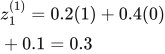 LaTeX:
z^{(1)}_1=0.2(1)+0.4(0)+0.1=0.3Step 3: calculate the second hidden preactivation.
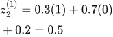 LaTeX:
z^{(1)}_2=0.3(1)+0.7(0)+0.2=0.5Step 4: activate the hidden layer. Both values are positive, so ReLU retains them.
 LaTeX:
a^{(1)}_1=\max(0,0.3)=0.3 LaTeX:
a^{(1)}_2=\max(0,0.5)=0.5 LaTeX:
a^{(1)}=\begin{bmatrix}0.3\\0.5\end{bmatrix}Step 5: calculate the output preactivation. Use the activated hidden values as this layer's inputs.
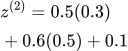 LaTeX:
z^{(2)}=0.5(0.3)+0.6(0.5)+0.1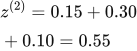 LaTeX:
z^{(2)}=0.15+0.30+0.10=0.55Step 6: apply the output activation.
 LaTeX:
\hat y=\max(0,0.55)=0.55Final answer: hidden preactivations and activations are [0.3, 0.5]ᵀ; output preactivation and prediction are both 0.55. They coincide here because every ReLU input is positive. No parameter has been updated during this forward pass.
Model answer: forward propagation, backpropagation and updating
Question
Question. Explain how a feedforward neural network learns using forward propagation, a loss function, backpropagation and gradient descent. State the order of operations.
Answer — step by step
Training repeatedly uses labeled examples to improve a network's weights and biases. The four operations have different jobs.
| Operation | Direction or action | Result |
|---|---|---|
| Forward propagation | Inputs move through successive layers | Predictions and intermediate activations |
| Loss calculation | Compare predictions with targets | A scalar objective for the example or batch |
| Backpropagation | Apply the chain rule from the loss toward earlier layers | Gradients of the objective with respect to parameters |
| Optimizer update | Use those gradients to change parameters | A new set of weights and biases |
1. Forward propagation
At each layer, calculate its weighted sums and activations. Retain these values because derivatives such as the sigmoid derivative depend on them. Complete a whole layer before calculating the next.
LaTeX: z^{(l)}=W^{(l)}a^{(l-1)}+b^{(l)},\qquad a^{(l)}=f(z^{(l)})2. Loss
Use the loss specified by the task. For one regression output, half squared loss is one possible choice:
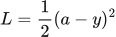 LaTeX:
L=\frac12(a-y)^2Here a is the prediction and y is the target. Other stated losses produce different derivatives.
3. Backpropagation
Multiply local derivatives along each dependency path. If a hidden unit influences several outputs, add the contributions from those branches. For a connection, the weight gradient is the receiving neuron's net-input derivative multiplied by the sending activation.
 LaTeX:
\frac{\partial L}{\partial w_{ji}}=\delta_j a_iHere δⱼ means the derivative of loss with respect to the receiving neuron's weighted sum. It is not automatically equal to raw prediction error; the activation and loss determine it.
4. Update and repeat
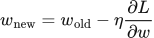 LaTeX:
w_{\mathrm{new}}=w_{\mathrm{old}}-\eta\frac{\partial L}{\partial w}Compute all gradients using the same pre-update weights. Then update the requested parameters. Run another forward pass to calculate the new loss. Backpropagation calculates gradients; gradient descent uses them. Those are related, separate operations.
Backpropagation with one hidden neuron
Definition. Backpropagation computes the derivatives of a scalar objective with respect to network parameters by applying the chain rule in reverse through the computational graph. An optimizer then uses these derivatives to update the parameters.
Network equations and the meaning of delta
Consider one input, one hidden neuron and one output neuron:
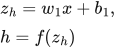 LaTeX:
z_h=w_1x+b_1,\qquad h=f(z_h)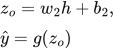 LaTeX:
z_o=w_2h+b_2,\qquad\hat y=g(z_o)For the half squared loss used in this example:
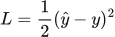 LaTeX:
L=\frac12(\hat y-y)^2Define a neuron's delta as the derivative of the loss with respect to its preactivation, not with respect to its output:
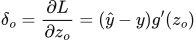 LaTeX:
\delta_o=\frac{\partial L}{\partial z_o}=(\hat y-y)g'(z_o)The output-weight derivative contains the hidden activation because zₒ = w₂h + b₂:
 LaTeX:
\frac{\partial L}{\partial w_2}=\delta_o h,\qquad\frac{\partial L}{\partial b_2}=\delta_oTo reach the hidden neuron, continue backwards through the old output weight and the hidden activation:
 LaTeX:
\delta_h=\delta_o w_2 f'(z_h) LaTeX:
\frac{\partial L}{\partial w_1}=\delta_h x,\qquad\frac{\partial L}{\partial b_1}=\delta_hThe bias derivative equals the corresponding delta because the derivative of z with respect to its additive bias is 1. All these derivatives belong to the same forward pass; an updated weight must not be used partway through this backward pass.
Complete worked numerical
Question. x = 2, y = 1; w₁ = 0.5, b₁ = 0.1; w₂ = 0.8, b₂ = 0.2. Both neurons use ReLU. Use half squared loss. Find the output and all four parameter gradients, then update all four parameters using η = 0.1.
Given
x = 2, y = 1.
w₁ = 0.5, b₁ = 0.1.
w₂ = 0.8, b₂ = 0.2.
Both neurons use ReLU.
Use half squared loss.
Find the output and all four parameter gradients, then update all four parameters using η = 0.1.
To find
Find all preactivations, hidden activations and final outputs. Calculate the half summed squared loss and its output derivatives. Find the requested deltas and parameter gradients, then update the specified parameters.
Formula — which one and why
Forward propagation. Evaluate one layer completely before supplying its activated outputs to the next layer. Each layer has its own weights and biases.
x = input vector; h = hidden outputs; W₁,b₁ = hidden parameters; W₂,b₂ = output parameters; f₁,f₂ = the stated activations.
LaTeX: z_h=W_1x+b_1LaTeX: h=f_1(z_h)LaTeX: z_o=W_2h+b_2LaTeX: o=f_2(z_o)Yaad rakhne ka cue: Pehli layer ka activated output hi agli layer ka input hai.
Half summed squared loss. This loss convention takes one-half of the sum of squared prediction errors. Use it when the question specifies it, or explicitly state it as an assumption when the paper omits the loss. Differentiating cancels the factor one-half against the square derivative.
oⱼ = output j; yⱼ = target j; L = half summed squared loss under the stated or explicitly assumed convention.
LaTeX: L=\frac12\sum_j(o_j-y_j)^2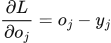 LaTeX:
\frac{\partial L}{\partial o_j}=o_j-y_jYaad rakhne ka cue: Half aur square ka 2 cancel: output derivative = prediction − target.
Backpropagation. The loss tells us how each output must change. Multiply by that neuron’s activation slope to obtain its delta. A weight gradient is receiving delta × sending value. Hidden deltas must include every outgoing path.
δ (delta) = derivative of loss with respect to a neuron’s preactivation; f′ = activation derivative; aᵢ = sending activation; Wⱼᵢ = connection weight. Use the exact loss scaling in the question.
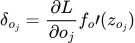 LaTeX:
\delta_{o_j}=\frac{\partial L}{\partial o_j}f_o\prime(z_{o_j})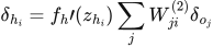 LaTeX:
\delta_{h_i}=f_h\prime(z_{h_i})\sum_jW_{ji}^{(2)}\delta_{o_j}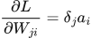 LaTeX:
\frac{\partial L}{\partial W_{ji}}=\delta_ja_i LaTeX:
\frac{\partial L}{\partial b_j}=\delta_j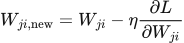 LaTeX:
W_{ji,\mathrm{new}}=W_{ji}-\eta\frac{\partial L}{\partial W_{ji}}Yaad rakhne ka cue: Receiving delta × sending value = us connection ka gradient.
Solution — step by step
Step 1: forward propagation through the hidden neuron.
 LaTeX:
z_h=0.5(2)+0.1=1.1 LaTeX:
h=\operatorname{ReLU}(1.1)=1.1Step 2: forward propagation through the output neuron.
 LaTeX:
z_o=0.8(1.1)+0.2=1.08 LaTeX:
\hat y=\operatorname{ReLU}(1.08)=1.08ReLU is not bounded above by 1, so this output is valid. It is not being interpreted as a probability here.
Step 3: calculate the loss and output delta.
 LaTeX:
L=\frac12(1.08-1)^2=0.0032Both preactivations are positive, so both ReLU derivatives are 1.
 LaTeX:
\delta_o=(1.08-1)(1)=0.08Step 4: calculate the output-layer parameter gradients.
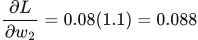 LaTeX:
\frac{\partial L}{\partial w_2}=0.08(1.1)=0.088 LaTeX:
\frac{\partial L}{\partial b_2}=0.08Step 5: propagate the derivative to the hidden neuron.
Use w₂ = 0.8, its value during the forward pass:
 LaTeX:
\delta_h=0.08(0.8)(1)=0.064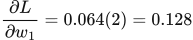 LaTeX:
\frac{\partial L}{\partial w_1}=0.064(2)=0.128 LaTeX:
\frac{\partial L}{\partial b_1}=0.064Step 6: update each parameter using its own gradient.
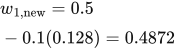 LaTeX:
w_{1,\mathrm{new}}=0.5-0.1(0.128)=0.4872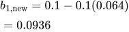 LaTeX:
b_{1,\mathrm{new}}=0.1-0.1(0.064)=0.0936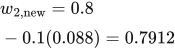 LaTeX:
w_{2,\mathrm{new}}=0.8-0.1(0.088)=0.7912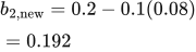 LaTeX:
b_{2,\mathrm{new}}=0.2-0.1(0.08)=0.192| Parameter | Gradient from the original forward pass | Updated value |
|---|---|---|
| w₁ | 0.128 | 0.4872 |
| b₁ | 0.064 | 0.0936 |
| w₂ | 0.088 | 0.7912 |
| b₂ | 0.08 | 0.192 |
Final answer: the original prediction is 1.08 and its loss is 0.0032. The table contains all requested gradients and updated parameters. A new forward pass would use all four new parameters together.
Drill 11 Full ReLU backpropagation
Question
Question. Input x = [1, 2]. Each row below lists the incoming weights of one receiving neuron. W₁ is shown below; b₁ = [0.1, 0.2]; W₂ is shown below; b₂ = [0.1]. Hidden and output activations are ReLU. Target y = [1]. Learning rate η = 0.1. Use half squared loss and update all weights and biases.
Answer — step by step
Given
Input x = [1, 2].
W₁ is printed with the question.
b₁ = [0.1, 0.2].
W₂ is printed with the question.
b₂ = [0.1].
Hidden and output activations are ReLU.
Target y = [1].
Learning rate η = 0.1.
Use half squared loss and update all weights and biases.
To find
Find all preactivations, hidden activations and final outputs. Calculate the half summed squared loss and its output derivatives. Find the requested deltas and parameter gradients, then update the specified parameters.
Formula — which one and why
Forward propagation. Evaluate one layer completely before supplying its activated outputs to the next layer. Each layer has its own weights and biases.
x = input vector; h = hidden outputs; W₁,b₁ = hidden parameters; W₂,b₂ = output parameters; f₁,f₂ = the stated activations.
LaTeX: z_h=W_1x+b_1LaTeX: h=f_1(z_h)LaTeX: z_o=W_2h+b_2LaTeX: o=f_2(z_o)Yaad rakhne ka cue: Pehli layer ka activated output hi agli layer ka input hai.
Half summed squared loss. This loss convention takes one-half of the sum of squared prediction errors. Use it when the question specifies it, or explicitly state it as an assumption when the paper omits the loss. Differentiating cancels the factor one-half against the square derivative.
oⱼ = output j; yⱼ = target j; L = half summed squared loss under the stated or explicitly assumed convention.
LaTeX: L=\frac12\sum_j(o_j-y_j)^2LaTeX: \frac{\partial L}{\partial o_j}=o_j-y_jYaad rakhne ka cue: Half aur square ka 2 cancel: output derivative = prediction − target.
Backpropagation. The loss tells us how each output must change. Multiply by that neuron’s activation slope to obtain its delta. A weight gradient is receiving delta × sending value. Hidden deltas must include every outgoing path.
δ (delta) = derivative of loss with respect to a neuron’s preactivation; f′ = activation derivative; aᵢ = sending activation; Wⱼᵢ = connection weight. Use the exact loss scaling in the question.
LaTeX: \delta_{o_j}=\frac{\partial L}{\partial o_j}f_o\prime(z_{o_j})LaTeX: \delta_{h_i}=f_h\prime(z_{h_i})\sum_jW_{ji}^{(2)}\delta_{o_j}LaTeX: \frac{\partial L}{\partial W_{ji}}=\delta_ja_iLaTeX: \frac{\partial L}{\partial b_j}=\delta_jLaTeX: W_{ji,\mathrm{new}}=W_{ji}-\eta\frac{\partial L}{\partial W_{ji}}Yaad rakhne ka cue: Receiving delta × sending value = us connection ka gradient.
Solution — step by step
Formulas used before substituting numbers
For every receiving neuron, z is its weighted sum and a is its activated output. The half squared loss sums the errors from all output neurons.
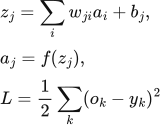 LaTeX:
z_j=\sum_iw_{ji}a_i+b_j,\quad a_j=f(z_j),\quad L=\frac12\sum_k(o_k-y_k)^2Delta means the loss gradient with respect to a neuron's raw score. First calculate output deltas, then hidden deltas using every connected output path.
 LaTeX:
\delta_{o_k}=(o_k-y_k)f'(z_{o_k})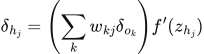 LaTeX:
\delta_{h_j}=\left(\sum_kw_{kj}\delta_{o_k}\right)f'(z_{h_j})The gradient of a connection is its receiving delta multiplied by its sending activation. A bias receives the constant 1.
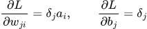 LaTeX:
\frac{\partial L}{\partial w_{ji}}=\delta_j a_i,\qquad \frac{\partial L}{\partial b_j}=\delta_j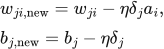 LaTeX:
w_{ji,\mathrm{new}}=w_{ji}-\eta\delta_j a_i,\quad b_{j,\mathrm{new}}=b_j-\eta\delta_jFor sigmoid, use f′ = a(1 − a). For ReLU, use f′ = 1 for a positive raw score and 0 for a negative raw score. Store the old weights until all gradients have been calculated.
Step 1 map the arrows. Each row of W₁ receives all inputs; each row of W₂ receives all hidden outputs. Bias is added once per receiving neuron. All gradients below use the OLD weights from this same forward pass.
Hidden neuron 1:
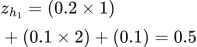 LaTeX:
z_{h_1} = (0.2 \times 1) + (0.1 \times 2) + (0.1) = 0.5 LaTeX:
h_{1} = \max(0,0.5) = 0.5Hidden neuron 2:
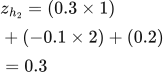 LaTeX:
z_{h_2} = (0.3 \times 1) + (-0.1 \times 2) + (0.2) = 0.3 LaTeX:
h_{2} = \max(0,0.3) = 0.3Output neuron 1:
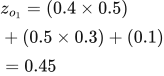 LaTeX:
z_{o_1} = (0.4 \times 0.5) + (0.5 \times 0.3) + (0.1) = 0.45 LaTeX:
o_{1} = \max(0,0.45) = 0.45Step 2 loss convention. This worked solution uses half summed squared loss, L = ½Σ(o − y)². Follow the loss specified in the question; where none is supplied, this is an explicit assumption.
Prediction minus target = [-0.55]. Squared errors = [0.3025]. Half-sum squared loss = 0.15125; mean squared error = 0.3025. These are different unless the number of output components makes the scale coincide.
Output delta 1:
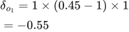 LaTeX:
\delta_{o_1} = 1 \times (0.45-1) \times 1 = -0.55The ReLU derivative is 1 here because this preactivation is positive.
Step 3 output weights. Gradient = receiving delta × sending activation. An output bias gradient equals its delta.
h1 → o1:
Subtract η × gradient = −0.0275. This weight increases.
The sending value and receiving delta have different roles. All deltas still use the original forward-pass weights.
The receiving neuron supplies the delta; the sending neuron supplies its activation.
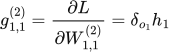 LaTeX:
g_{1,1}^{(2)}=\frac{\partial L}{\partial W^{(2)}_{1,1}}=\delta_{o_1}h_1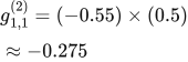 LaTeX:
g_{1,1}^{(2)}=(-0.55)\times(0.5)\approx -0.275Apply the learning rate to this gradient and subtract the result from the old weight.
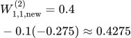 LaTeX:
W^{(2)}_{1,1,\mathrm{new}}=0.4-0.1(-0.275)\approx 0.4275h2 → o1:
Subtract η × gradient = −0.0165. This weight increases.
The sending value and receiving delta have different roles. All deltas still use the original forward-pass weights.
The receiving neuron supplies the delta; the sending neuron supplies its activation.
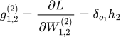 LaTeX:
g_{1,2}^{(2)}=\frac{\partial L}{\partial W^{(2)}_{1,2}}=\delta_{o_1}h_2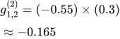 LaTeX:
g_{1,2}^{(2)}=(-0.55)\times(0.3)\approx -0.165Apply the learning rate to this gradient and subtract the result from the old weight.
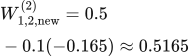 LaTeX:
W^{(2)}_{1,2,\mathrm{new}}=0.5-0.1(-0.165)\approx 0.5165Step 4 hidden deltas. A hidden unit can influence EVERY connected output, so add those paths BEFORE multiplying by the hidden activation derivative.
Hidden 1 downstream contribution:
Calculate each outgoing path using the old outgoing weight and that output's delta.
Multiply within each path. Add the resulting contributions at the shared hidden neuron.
Contribution from output 1.
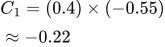 LaTeX:
C_1=(0.4)\times(-0.55)\approx -0.22Accumulate the contributions, then apply the hidden activation derivative below.
 LaTeX:
\text{Sum}=C_1\approx -0.22 LaTeX:
\delta_{h_1} = -0.22 \times 1 = -0.22Hidden 2 downstream contribution:
Calculate each outgoing path using the old outgoing weight and that output's delta.
Multiply within each path. Add the resulting contributions at the shared hidden neuron.
Contribution from output 1.
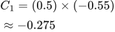 LaTeX:
C_1=(0.5)\times(-0.55)\approx -0.275Accumulate the contributions, then apply the hidden activation derivative below.
 LaTeX:
\text{Sum}=C_1\approx -0.275 LaTeX:
\delta_{h_2} = -0.275 \times 1 = -0.275Step 5 input weights. Multiply the hidden delta by the corresponding raw input, not by the hidden output.
x1 → h1:
Subtract η × gradient = −0.022. This weight increases.
The sending value and receiving delta have different roles. All deltas still use the original forward-pass weights.
The receiving neuron supplies the delta; the sending neuron supplies the input value.
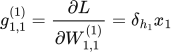 LaTeX:
g_{1,1}^{(1)}=\frac{\partial L}{\partial W^{(1)}_{1,1}}=\delta_{h_1}x_1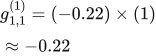 LaTeX:
g_{1,1}^{(1)}=(-0.22)\times(1)\approx -0.22Apply the learning rate to this gradient and subtract the result from the old weight.
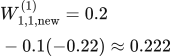 LaTeX:
W^{(1)}_{1,1,\mathrm{new}}=0.2-0.1(-0.22)\approx 0.222x2 → h1:
Subtract η × gradient = −0.044. This weight increases.
The sending value and receiving delta have different roles. All deltas still use the original forward-pass weights.
The receiving neuron supplies the delta; the sending neuron supplies the input value.
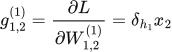 LaTeX:
g_{1,2}^{(1)}=\frac{\partial L}{\partial W^{(1)}_{1,2}}=\delta_{h_1}x_2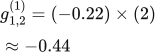 LaTeX:
g_{1,2}^{(1)}=(-0.22)\times(2)\approx -0.44Apply the learning rate to this gradient and subtract the result from the old weight.
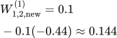 LaTeX:
W^{(1)}_{1,2,\mathrm{new}}=0.1-0.1(-0.44)\approx 0.144x1 → h2:
Subtract η × gradient = −0.0275. This weight increases.
The sending value and receiving delta have different roles. All deltas still use the original forward-pass weights.
The receiving neuron supplies the delta; the sending neuron supplies the input value.
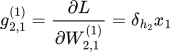 LaTeX:
g_{2,1}^{(1)}=\frac{\partial L}{\partial W^{(1)}_{2,1}}=\delta_{h_2}x_1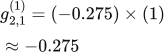 LaTeX:
g_{2,1}^{(1)}=(-0.275)\times(1)\approx -0.275Apply the learning rate to this gradient and subtract the result from the old weight.
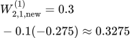 LaTeX:
W^{(1)}_{2,1,\mathrm{new}}=0.3-0.1(-0.275)\approx 0.3275x2 → h2:
Subtract η × gradient = −0.055. This weight increases.
The sending value and receiving delta have different roles. All deltas still use the original forward-pass weights.
The receiving neuron supplies the delta; the sending neuron supplies the input value.
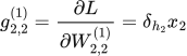 LaTeX:
g_{2,2}^{(1)}=\frac{\partial L}{\partial W^{(1)}_{2,2}}=\delta_{h_2}x_2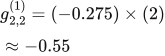 LaTeX:
g_{2,2}^{(1)}=(-0.275)\times(2)\approx -0.55Apply the learning rate to this gradient and subtract the result from the old weight.
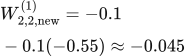 LaTeX:
W^{(1)}_{2,2,\mathrm{new}}=-0.1-0.1(-0.55)\approx -0.045Step 6 bias updates. A bias receives a constant input 1, so its gradient equals the corresponding delta. Use the same old forward pass and learning rate as the weight updates.
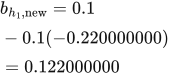 LaTeX:
b_{h_1,\mathrm{new}}=0.1-0.1(-0.220000000)=0.122000000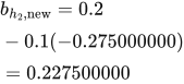 LaTeX:
b_{h_2,\mathrm{new}}=0.2-0.1(-0.275000000)=0.227500000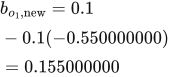 LaTeX:
b_{o_1,\mathrm{new}}=0.1-0.1(-0.550000000)=0.155000000These are independent per-neuron biases. If the question fixes biases, keep them fixed. If it specifies a single tied bias, add all deltas sharing that bias before updating it.
Drill 12 Two output sigmoid backpropagation
Question
Question. Input x = [0.2, 0.4]. Each row below lists the incoming weights of one receiving neuron. W₁ is shown below; b₁ = [0.1, 0.1]; W₂ is shown below; b₂ = [0, 0.1]. Hidden and output activations are sigmoid. Target y = [1, 0]. Learning rate η = 0.2. Use half summed squared loss and update all parameters.
Answer — step by step
Given
Input x = [0.2, 0.4].
W₁ is printed with the question.
b₁ = [0.1, 0.1].
W₂ is printed with the question.
b₂ = [0, 0.1].
Hidden and output activations are sigmoid.
Target y = [1, 0].
Learning rate η = 0.2.
Use half summed squared loss and update all parameters.
To find
Find all preactivations, hidden activations and final outputs. Calculate the half summed squared loss and its output derivatives. Find the sigmoid output and, if requested, its derivative. Find the requested deltas and parameter gradients, then update the specified parameters.
Formula — which one and why
Forward propagation. Evaluate one layer completely before supplying its activated outputs to the next layer. Each layer has its own weights and biases.
x = input vector; h = hidden outputs; W₁,b₁ = hidden parameters; W₂,b₂ = output parameters; f₁,f₂ = the stated activations.
LaTeX: z_h=W_1x+b_1LaTeX: h=f_1(z_h)LaTeX: z_o=W_2h+b_2LaTeX: o=f_2(z_o)Yaad rakhne ka cue: Pehli layer ka activated output hi agli layer ka input hai.
Half summed squared loss. This loss convention takes one-half of the sum of squared prediction errors. Use it when the question specifies it, or explicitly state it as an assumption when the paper omits the loss. Differentiating cancels the factor one-half against the square derivative.
oⱼ = output j; yⱼ = target j; L = half summed squared loss under the stated or explicitly assumed convention.
LaTeX: L=\frac12\sum_j(o_j-y_j)^2LaTeX: \frac{\partial L}{\partial o_j}=o_j-y_jYaad rakhne ka cue: Half aur square ka 2 cancel: output derivative = prediction − target.
Sigmoid and its slope. Use sigmoid when the neuron is specified to squash its preactivation into (0,1). Once its output is known, its derivative needs only output × (1−output).
z = preactivation; p = sigmoid output; e is the exponential base, not a prediction error in this formula.
 LaTeX:
p=\frac{1}{1+e^{-z}}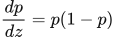 LaTeX:
\frac{dp}{dz}=p(1-p)Yaad rakhne ka cue: Sigmoid output p; uska slope p × (1−p).
Backpropagation. The loss tells us how each output must change. Multiply by that neuron’s activation slope to obtain its delta. A weight gradient is receiving delta × sending value. Hidden deltas must include every outgoing path.
δ (delta) = derivative of loss with respect to a neuron’s preactivation; f′ = activation derivative; aᵢ = sending activation; Wⱼᵢ = connection weight. Use the exact loss scaling in the question.
LaTeX: \delta_{o_j}=\frac{\partial L}{\partial o_j}f_o\prime(z_{o_j})LaTeX: \delta_{h_i}=f_h\prime(z_{h_i})\sum_jW_{ji}^{(2)}\delta_{o_j}LaTeX: \frac{\partial L}{\partial W_{ji}}=\delta_ja_iLaTeX: \frac{\partial L}{\partial b_j}=\delta_jLaTeX: W_{ji,\mathrm{new}}=W_{ji}-\eta\frac{\partial L}{\partial W_{ji}}Yaad rakhne ka cue: Receiving delta × sending value = us connection ka gradient.
Solution — step by step
Formulas used before substituting numbers
For every receiving neuron, z is its weighted sum and a is its activated output. The half squared loss sums the errors from all output neurons.
LaTeX: z_j=\sum_iw_{ji}a_i+b_j,\quad a_j=f(z_j),\quad L=\frac12\sum_k(o_k-y_k)^2Delta means the loss gradient with respect to a neuron's raw score. First calculate output deltas, then hidden deltas using every connected output path.
LaTeX: \delta_{o_k}=(o_k-y_k)f'(z_{o_k})LaTeX: \delta_{h_j}=\left(\sum_kw_{kj}\delta_{o_k}\right)f'(z_{h_j})The gradient of a connection is its receiving delta multiplied by its sending activation. A bias receives the constant 1.
LaTeX: \frac{\partial L}{\partial w_{ji}}=\delta_j a_i,\qquad \frac{\partial L}{\partial b_j}=\delta_jLaTeX: w_{ji,\mathrm{new}}=w_{ji}-\eta\delta_j a_i,\quad b_{j,\mathrm{new}}=b_j-\eta\delta_jFor sigmoid, use f′ = a(1 − a). For ReLU, use f′ = 1 for a positive raw score and 0 for a negative raw score. Store the old weights until all gradients have been calculated.
Step 1 map the arrows. Each row of W₁ receives all inputs; each row of W₂ receives all hidden outputs. Bias is added once per receiving neuron. All gradients below use the OLD weights from this same forward pass.
Hidden neuron 1:
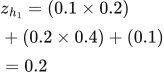 LaTeX:
z_{h_1} = (0.1 \times 0.2) + (0.2 \times 0.4) + (0.1) = 0.2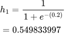 LaTeX:
h_{1}=\frac{1}{1+e^{-(0.2)}}=0.549833997Hidden neuron 2:
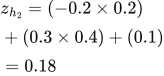 LaTeX:
z_{h_2} = (-0.2 \times 0.2) + (0.3 \times 0.4) + (0.1) = 0.18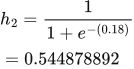 LaTeX:
h_{2}=\frac{1}{1+e^{-(0.18)}}=0.544878892Output neuron 1:
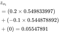 LaTeX:
z_{o_1} = (0.2 \times 0.549833997) + (-0.1 \times 0.544878892) + (0) = 0.05547891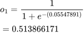 LaTeX:
o_{1}=\frac{1}{1+e^{-(0.05547891)}}=0.513866171Output neuron 2:
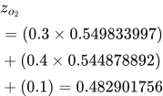 LaTeX:
z_{o_2} = (0.3 \times 0.549833997) + (0.4 \times 0.544878892) + (0.1) = 0.482901756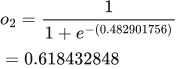 LaTeX:
o_{2}=\frac{1}{1+e^{-(0.482901756)}}=0.618432848Step 2 loss convention. This worked solution uses half summed squared loss, L = ½Σ(o − y)². Follow the loss specified in the question; where none is supplied, this is an explicit assumption.
Prediction minus target = [-0.486133829, 0.618432848]. Squared errors = [0.2363261, 0.382459187]. Half-sum squared loss = 0.309392643; mean squared error = 0.309392643. These are different unless the number of output components makes the scale coincide.
Output delta 1:
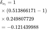 LaTeX:
\delta_{o_1} = 1 \times (0.513866171-1) \times 0.249807729 = -0.121439988The derivative is o(1−o).
Output delta 2:
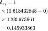 LaTeX:
\delta_{o_2} = 1 \times (0.618432848-0) \times 0.235973661 = 0.145933863The derivative is o(1−o).
Step 3 output weights. Gradient = receiving delta × sending activation. An output bias gradient equals its delta.
h1 → o1:
Subtract η × gradient = −0.013354367. This weight increases.
The sending value and receiving delta have different roles. All deltas still use the original forward-pass weights.
The receiving neuron supplies the delta; the sending neuron supplies its activation.
LaTeX: g_{1,1}^{(2)}=\frac{\partial L}{\partial W^{(2)}_{1,1}}=\delta_{o_1}h_1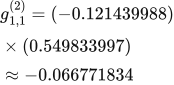 LaTeX:
g_{1,1}^{(2)}=(-0.121439988)\times(0.549833997)\approx -0.066771834Apply the learning rate to this gradient and subtract the result from the old weight.
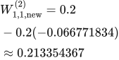 LaTeX:
W^{(2)}_{1,1,\mathrm{new}}=0.2-0.2(-0.066771834)\approx 0.213354367h2 → o1:
Subtract η × gradient = −0.013234017. This weight increases.
The sending value and receiving delta have different roles. All deltas still use the original forward-pass weights.
The receiving neuron supplies the delta; the sending neuron supplies its activation.
LaTeX: g_{1,2}^{(2)}=\frac{\partial L}{\partial W^{(2)}_{1,2}}=\delta_{o_1}h_2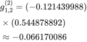 LaTeX:
g_{1,2}^{(2)}=(-0.121439988)\times(0.544878892)\approx -0.066170086Apply the learning rate to this gradient and subtract the result from the old weight.
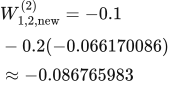 LaTeX:
W^{(2)}_{1,2,\mathrm{new}}=-0.1-0.2(-0.066170086)\approx -0.086765983h1 → o2:
Subtract η × gradient = 0.01604788. This weight decreases.
The sending value and receiving delta have different roles. All deltas still use the original forward-pass weights.
The receiving neuron supplies the delta; the sending neuron supplies its activation.
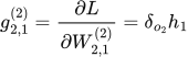 LaTeX:
g_{2,1}^{(2)}=\frac{\partial L}{\partial W^{(2)}_{2,1}}=\delta_{o_2}h_1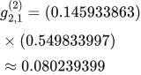 LaTeX:
g_{2,1}^{(2)}=(0.145933863)\times(0.549833997)\approx 0.080239399Apply the learning rate to this gradient and subtract the result from the old weight.
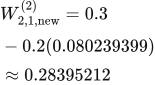 LaTeX:
W^{(2)}_{2,1,\mathrm{new}}=0.3-0.2(0.080239399)\approx 0.28395212h2 → o2:
Subtract η × gradient = 0.015903256. This weight decreases.
The sending value and receiving delta have different roles. All deltas still use the original forward-pass weights.
The receiving neuron supplies the delta; the sending neuron supplies its activation.
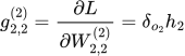 LaTeX:
g_{2,2}^{(2)}=\frac{\partial L}{\partial W^{(2)}_{2,2}}=\delta_{o_2}h_2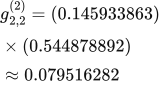 LaTeX:
g_{2,2}^{(2)}=(0.145933863)\times(0.544878892)\approx 0.079516282Apply the learning rate to this gradient and subtract the result from the old weight.
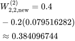 LaTeX:
W^{(2)}_{2,2,\mathrm{new}}=0.4-0.2(0.079516282)\approx 0.384096744Step 4 hidden deltas. A hidden unit can influence EVERY connected output, so add those paths BEFORE multiplying by the hidden activation derivative.
Hidden 1 downstream contribution:
Calculate each outgoing path using the old outgoing weight and that output's delta.
Multiply within each path. Add the resulting contributions at the shared hidden neuron.
Contribution from output 1.
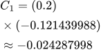 LaTeX:
C_1=(0.2)\times(-0.121439988)\approx -0.024287998Contribution from output 2.
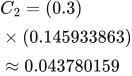 LaTeX:
C_2=(0.3)\times(0.145933863)\approx 0.043780159Accumulate the contributions, then apply the hidden activation derivative below.
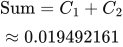 LaTeX:
\text{Sum}=C_1+C_2\approx 0.019492161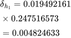 LaTeX:
\delta_{h_1} = 0.019492161 \times 0.247516573 = 0.004824633Hidden 2 downstream contribution:
Calculate each outgoing path using the old outgoing weight and that output's delta.
Multiply within each path. Add the resulting contributions at the shared hidden neuron.
Contribution from output 1.
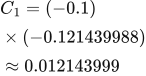 LaTeX:
C_1=(-0.1)\times(-0.121439988)\approx 0.012143999Contribution from output 2.
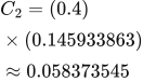 LaTeX:
C_2=(0.4)\times(0.145933863)\approx 0.058373545Accumulate the contributions, then apply the hidden activation derivative below.
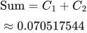 LaTeX:
\text{Sum}=C_1+C_2\approx 0.070517544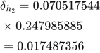 LaTeX:
\delta_{h_2} = 0.070517544 \times 0.247985885 = 0.017487356Step 5 input weights. Multiply the hidden delta by the corresponding raw input, not by the hidden output.
x1 → h1:
Subtract η × gradient = 0.000192985. This weight decreases.
The sending value and receiving delta have different roles. All deltas still use the original forward-pass weights.
The receiving neuron supplies the delta; the sending neuron supplies the input value.
LaTeX: g_{1,1}^{(1)}=\frac{\partial L}{\partial W^{(1)}_{1,1}}=\delta_{h_1}x_1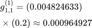 LaTeX:
g_{1,1}^{(1)}=(0.004824633)\times(0.2)\approx 0.000964927Apply the learning rate to this gradient and subtract the result from the old weight.
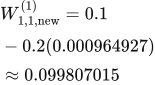 LaTeX:
W^{(1)}_{1,1,\mathrm{new}}=0.1-0.2(0.000964927)\approx 0.099807015x2 → h1:
Subtract η × gradient = 0.000385971. This weight decreases.
The sending value and receiving delta have different roles. All deltas still use the original forward-pass weights.
The receiving neuron supplies the delta; the sending neuron supplies the input value.
LaTeX: g_{1,2}^{(1)}=\frac{\partial L}{\partial W^{(1)}_{1,2}}=\delta_{h_1}x_2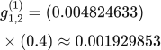 LaTeX:
g_{1,2}^{(1)}=(0.004824633)\times(0.4)\approx 0.001929853Apply the learning rate to this gradient and subtract the result from the old weight.
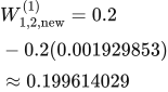 LaTeX:
W^{(1)}_{1,2,\mathrm{new}}=0.2-0.2(0.001929853)\approx 0.199614029x1 → h2:
Subtract η × gradient = 0.000699494. This weight decreases.
The sending value and receiving delta have different roles. All deltas still use the original forward-pass weights.
The receiving neuron supplies the delta; the sending neuron supplies the input value.
LaTeX: g_{2,1}^{(1)}=\frac{\partial L}{\partial W^{(1)}_{2,1}}=\delta_{h_2}x_1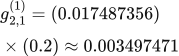 LaTeX:
g_{2,1}^{(1)}=(0.017487356)\times(0.2)\approx 0.003497471Apply the learning rate to this gradient and subtract the result from the old weight.
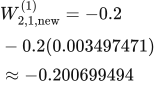 LaTeX:
W^{(1)}_{2,1,\mathrm{new}}=-0.2-0.2(0.003497471)\approx -0.200699494x2 → h2:
Subtract η × gradient = 0.001398988. This weight decreases.
The sending value and receiving delta have different roles. All deltas still use the original forward-pass weights.
The receiving neuron supplies the delta; the sending neuron supplies the input value.
LaTeX: g_{2,2}^{(1)}=\frac{\partial L}{\partial W^{(1)}_{2,2}}=\delta_{h_2}x_2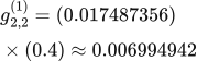 LaTeX:
g_{2,2}^{(1)}=(0.017487356)\times(0.4)\approx 0.006994942Apply the learning rate to this gradient and subtract the result from the old weight.
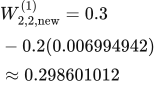 LaTeX:
W^{(1)}_{2,2,\mathrm{new}}=0.3-0.2(0.006994942)\approx 0.298601012Step 6 bias updates. A bias receives a constant input 1, so its gradient equals the corresponding delta. Use the same old forward pass and learning rate as the weight updates.
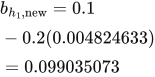 LaTeX:
b_{h_1,\mathrm{new}}=0.1-0.2(0.004824633)=0.099035073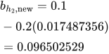 LaTeX:
b_{h_2,\mathrm{new}}=0.1-0.2(0.017487356)=0.096502529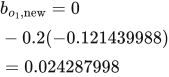 LaTeX:
b_{o_1,\mathrm{new}}=0-0.2(-0.121439988)=0.024287998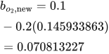 LaTeX:
b_{o_2,\mathrm{new}}=0.1-0.2(0.145933863)=0.070813227These are independent per-neuron biases. If the question fixes biases, keep them fixed. If it specifies a single tied bias, add all deltas sharing that bias before updating it.
Sigmoid and its derivative
Sigmoid takes a raw score and changes it to a number between 0 and 1. Its derivative is a different number: it tells backpropagation how sensitive that output is to its raw score. The complete example below calculates both and shows where each is used.
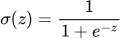 LaTeX:
\sigma(z)=\frac{1}{1+e^{-z}} LaTeX:
\sigma\prime(z)=\sigma(z)[1-\sigma(z)]Complete sigmoid training example
Question. A sigmoid neuron has input 2, weight 0, bias 0, target 1 and half squared loss. Will gradient descent increase or decrease the weight? Use learning rate 0.1 and calculate the exact update.
Given
x = 2; w = 0; b = 0; y = 1.
Sigmoid output; half squared loss; η = 0.1.
To find
Find the weight-gradient sign, exact weight update and resulting weight.
Formula — which one and why
Weighted sum and activation. Each input is multiplied by its connection weight. Add these contributions, add the bias once, then apply the stated activation.
xᵢ = input i; wᵢ = its weight; b = bias; z = sum before activation; a = output after activation; f = the specified activation function.
LaTeX: z=\sum_iw_ix_i+bLaTeX: a=f(z)Yaad rakhne ka cue: Input × weight, sabka sum, bias once, phir activation.
Sigmoid and its slope. Use sigmoid when the neuron is specified to squash its preactivation into (0,1). Once its output is known, its derivative needs only output × (1−output).
z = preactivation; p = sigmoid output; e is the exponential base, not a prediction error in this formula.
LaTeX: p=\frac{1}{1+e^{-z}}LaTeX: \frac{dp}{dz}=p(1-p)Yaad rakhne ka cue: Sigmoid output p; uska slope p × (1−p).
Half summed squared loss. This loss convention takes one-half of the sum of squared prediction errors. Use it when the question specifies it, or explicitly state it as an assumption when the paper omits the loss. Differentiating cancels the factor one-half against the square derivative.
oⱼ = output j; yⱼ = target j; L = half summed squared loss under the stated or explicitly assumed convention.
LaTeX: L=\frac12\sum_j(o_j-y_j)^2LaTeX: \frac{\partial L}{\partial o_j}=o_j-y_jYaad rakhne ka cue: Half aur square ka 2 cancel: output derivative = prediction − target.
Backpropagation. The loss tells us how each output must change. Multiply by that neuron’s activation slope to obtain its delta. A weight gradient is receiving delta × sending value. Hidden deltas must include every outgoing path.
δ (delta) = derivative of loss with respect to a neuron’s preactivation; f′ = activation derivative; aᵢ = sending activation; Wⱼᵢ = connection weight. Use the exact loss scaling in the question.
LaTeX: \delta_{o_j}=\frac{\partial L}{\partial o_j}f_o\prime(z_{o_j})LaTeX: \delta_{h_i}=f_h\prime(z_{h_i})\sum_jW_{ji}^{(2)}\delta_{o_j}LaTeX: \frac{\partial L}{\partial W_{ji}}=\delta_ja_iLaTeX: \frac{\partial L}{\partial b_j}=\delta_jLaTeX: W_{ji,\mathrm{new}}=W_{ji}-\eta\frac{\partial L}{\partial W_{ji}}Yaad rakhne ka cue: Receiving delta × sending value = us connection ka gradient.
Solution — step by step
Step 1 forward: net = 0(2) + 0 = 0; sigmoid output = 0.5.
Step 2 backward: prediction minus target = 0.5 − 1 = −0.5. Sigmoid slope = 0.5(1 − 0.5) = 0.25. Delta = −0.5 × 0.25 = −0.125.
Step 3 gradients and update: weight gradient = −0.125 × 2 = −0.25. New weight = 0 − 0.1(−0.25) = 0.025. Bias gradient = −0.125; new bias = 0.0125. Both increase. With positive input, these changes initially raise the prediction toward the target. Your intuition and arithmetic now agree.
Drill 10 Sigmoid neuron gradient
Question
Question. x = 2, w = 0.5, b = 0, y = 1, half squared loss, η = 0.1. Find one weight and bias update.
Answer — step by step
Given
x = 2; w = 0.5; b = 0; target y = 1.
Activation: sigmoid; loss: half squared error.
Learning rate η = 0.1.
To find
Find the output, delta, weight/bias gradients and one update.
Formula — which one and why
Weighted sum and activation. Each input is multiplied by its connection weight. Add these contributions, add the bias once, then apply the stated activation.
xᵢ = input i; wᵢ = its weight; b = bias; z = sum before activation; a = output after activation; f = the specified activation function.
LaTeX: z=\sum_iw_ix_i+bLaTeX: a=f(z)Yaad rakhne ka cue: Input × weight, sabka sum, bias once, phir activation.
Sigmoid and its slope. Use sigmoid when the neuron is specified to squash its preactivation into (0,1). Once its output is known, its derivative needs only output × (1−output).
z = preactivation; p = sigmoid output; e is the exponential base, not a prediction error in this formula.
LaTeX: p=\frac{1}{1+e^{-z}}LaTeX: \frac{dp}{dz}=p(1-p)Yaad rakhne ka cue: Sigmoid output p; uska slope p × (1−p).
Half summed squared loss. This loss convention takes one-half of the sum of squared prediction errors. Use it when the question specifies it, or explicitly state it as an assumption when the paper omits the loss. Differentiating cancels the factor one-half against the square derivative.
oⱼ = output j; yⱼ = target j; L = half summed squared loss under the stated or explicitly assumed convention.
LaTeX: L=\frac12\sum_j(o_j-y_j)^2LaTeX: \frac{\partial L}{\partial o_j}=o_j-y_jYaad rakhne ka cue: Half aur square ka 2 cancel: output derivative = prediction − target.
Backpropagation. The loss tells us how each output must change. Multiply by that neuron’s activation slope to obtain its delta. A weight gradient is receiving delta × sending value. Hidden deltas must include every outgoing path.
δ (delta) = derivative of loss with respect to a neuron’s preactivation; f′ = activation derivative; aᵢ = sending activation; Wⱼᵢ = connection weight. Use the exact loss scaling in the question.
LaTeX: \delta_{o_j}=\frac{\partial L}{\partial o_j}f_o\prime(z_{o_j})LaTeX: \delta_{h_i}=f_h\prime(z_{h_i})\sum_jW_{ji}^{(2)}\delta_{o_j}LaTeX: \frac{\partial L}{\partial W_{ji}}=\delta_ja_iLaTeX: \frac{\partial L}{\partial b_j}=\delta_jLaTeX: W_{ji,\mathrm{new}}=W_{ji}-\eta\frac{\partial L}{\partial W_{ji}}Yaad rakhne ka cue: Receiving delta × sending value = us connection ka gradient.
Solution — step by step
Meaning and formulas
Here the loss is half squared error. It is different from binary cross-entropy, so we include the sigmoid derivative explicitly.
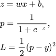 LaTeX:
z=wx+b,\quad p=\frac1{1+e^{-z}},\quad L=\frac12(p-y)^2The symbol δ (delta) is a short name for the loss gradient with respect to the neuron's raw score z.
 LaTeX:
\delta=(p-y)p(1-p)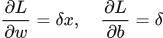 LaTeX:
\frac{\partial L}{\partial w}=\delta x,\quad \frac{\partial L}{\partial b}=\delta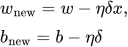 LaTeX:
w_{\mathrm{new}}=w-\eta\delta x,\quad b_{\mathrm{new}}=b-\eta\deltaStep 1: weighted sum and sigmoid
 LaTeX:
z=0.5\times2+0=1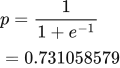 LaTeX:
p=\frac1{1+e^{-1}}=0.731058579Step 2: error and activation slope
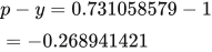 LaTeX:
p-y=0.731058579-1=-0.268941421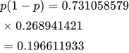 LaTeX:
p(1-p)=0.731058579\times0.268941421=0.196611933Step 3: multiply the linked effects to obtain delta
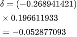 LaTeX:
\delta=(-0.268941421)\times0.196611933=-0.052877093Step 4: multiply delta by the input to each parameter
The weight receives x = 2. The bias effectively receives the constant input 1.
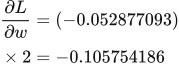 LaTeX:
\frac{\partial L}{\partial w}=(-0.052877093)\times2=-0.105754186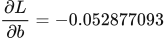 LaTeX:
\frac{\partial L}{\partial b}=-0.052877093Step 5: subtract learning rate times each gradient
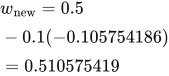 LaTeX:
w_{\mathrm{new}}=0.5-0.1(-0.105754186)=0.510575419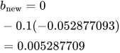 LaTeX:
b_{\mathrm{new}}=0-0.1(-0.052877093)=0.005287709Final answer: new weight ≈ 0.510575419; new bias ≈ 0.005287709. Subtracting negative gradients increases both values here.
sigmoid example 1
Question. For preactivation z = -2, calculate the sigmoid output and state its derivative.
Given
z = -2; activation = sigmoid.
To find
The output a and the derivative with respect to z.
Formula — which one and why
Use the activation named in the question. The derivative is a second calculation required for a backward pass.
z is the raw sum; a is the activated output; f′(z) is the local slope.
LaTeX: a=\frac1{1+e^{-z}} LaTeX:
f\prime(z)=a(1-a)Yaad rakhne ka cue: One over one plus e ki minus-z power; slope = output × (1−output).
Solution — step by step
Step 1: negate the whole input.
 LaTeX:
-z=-(-2)=2Step 2: calculate the exponential.
 LaTeX:
e^{2}\approx7.389056099Step 3: add one in the denominator.
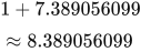 LaTeX:
1+7.389056099\approx8.389056099Step 4: divide one by the complete denominator.
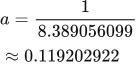 LaTeX:
a=\frac1{8.389056099}\approx0.119202922Step 5: use the activated output in the slope.
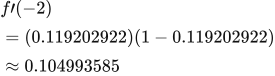 LaTeX:
f\prime(-2)=(0.119202922)(1-0.119202922)\approx0.104993585Final answer: a ≈ 0.119202922. Derivative ≈ 0.104993585.
sigmoid example 2
Question. For preactivation z = 0, calculate the sigmoid output and state its derivative.
Given
z = 0; activation = sigmoid.
To find
The output a and the derivative with respect to z.
Formula — which one and why
Use the activation named in the question. The derivative is a second calculation required for a backward pass.
z is the raw sum; a is the activated output; f′(z) is the local slope.
LaTeX: a=\frac1{1+e^{-z}}LaTeX: f\prime(z)=a(1-a)Yaad rakhne ka cue: One over one plus e ki minus-z power; slope = output × (1−output).
Solution — step by step
Step 1: negate the whole input.
 LaTeX:
-z=-(0)=0Step 2: calculate the exponential.
 LaTeX:
e^{0}\approx1.000000000Step 3: add one in the denominator.
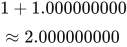 LaTeX:
1+1.000000000\approx2.000000000Step 4: divide one by the complete denominator.
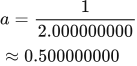 LaTeX:
a=\frac1{2.000000000}\approx0.500000000Step 5: use the activated output in the slope.
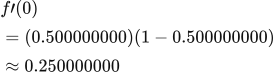 LaTeX:
f\prime(0)=(0.500000000)(1-0.500000000)\approx0.250000000Final answer: a ≈ 0.500000000. Derivative ≈ 0.250000000.
sigmoid example 3
Question. For preactivation z = 2, calculate the sigmoid output and state its derivative.
Given
z = 2; activation = sigmoid.
To find
The output a and the derivative with respect to z.
Formula — which one and why
Use the activation named in the question. The derivative is a second calculation required for a backward pass.
z is the raw sum; a is the activated output; f′(z) is the local slope.
LaTeX: a=\frac1{1+e^{-z}}LaTeX: f\prime(z)=a(1-a)Yaad rakhne ka cue: One over one plus e ki minus-z power; slope = output × (1−output).
Solution — step by step
Step 1: negate the whole input.
 LaTeX:
-z=-(2)=-2Step 2: calculate the exponential.
 LaTeX:
e^{-2}\approx0.135335283Step 3: add one in the denominator.
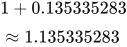 LaTeX:
1+0.135335283\approx1.135335283Step 4: divide one by the complete denominator.
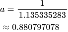 LaTeX:
a=\frac1{1.135335283}\approx0.880797078Step 5: use the activated output in the slope.
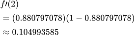 LaTeX:
f\prime(2)=(0.880797078)(1-0.880797078)\approx0.104993585Final answer: a ≈ 0.880797078. Derivative ≈ 0.104993585.
Tanh and its derivative
Tanh can produce a negative or positive output. In the formula, calculate the exponential first, then form the top and bottom of the fraction separately. The derivative uses the activated answer, not the raw input.
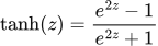 LaTeX:
\tanh(z)=\frac{e^{2z}-1}{e^{2z}+1} LaTeX:
\tanh\prime(z)=1-\tanh^2(z)Question. Calculate tanh(0.5) and its derivative with respect to the input.
Given
z = 0.5.
To find
Find tanh(z) and its derivative.
Formula — which one and why
Tanh and its slope. Tanh preserves a signed output between −1 and 1. Once its output a is known, the local slope is 1−a².
z = value entering tanh; a = its output. A prime means derivative, or local rate of change.
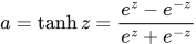 LaTeX:
a=\tanh z=\frac{e^z-e^{-z}}{e^z+e^{-z}}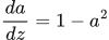 LaTeX:
\frac{da}{dz}=1-a^2Yaad rakhne ka cue: Tanh signed output deta hai; slope = 1 minus output ka square.
Solution — step by step
Step 1: identify the input. The input z is 0.5. In this version of the tanh formula, the exponential uses 2z.
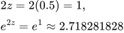 LaTeX:
2z=2(0.5)=1,\qquad e^{2z}=e^1\approx2.718281828Step 2: calculate the numerator. Subtract 1 from that exponential.
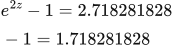 LaTeX:
e^{2z}-1=2.718281828-1=1.718281828Step 3: calculate the denominator. Add 1 to the same exponential.
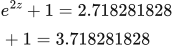 LaTeX:
e^{2z}+1=2.718281828+1=3.718281828Step 4: divide the top by the bottom.
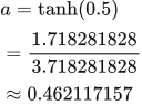 LaTeX:
a=\tanh(0.5)=\frac{1.718281828}{3.718281828}\approx0.462117157Step 5: calculate the local derivative. Square the output a and subtract it from 1. Keep the calculator's unrounded result.
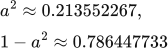 LaTeX:
a^2\approx0.213552267,\qquad1-a^2\approx0.786447733Final answer: tanh output ≈ 0.462117157; local derivative ≈ 0.786447733. The output becomes the next layer's input; the derivative is used when carrying a gradient backward.
tanh example 1
Question. For preactivation z = -2, calculate the tanh output and state its derivative.
Given
z = -2; activation = tanh.
To find
The output a and the derivative with respect to z.
Formula — which one and why
Use the activation named in the question. The derivative is a second calculation required for a backward pass.
z is the raw sum; a is the activated output; f′(z) is the local slope.
 LaTeX:
a=\frac{e^{2z}-1}{e^{2z}+1} LaTeX:
f\prime(z)=1-a^2Yaad rakhne ka cue: Tanh ka answer −1 se 1; slope one minus output squared.
Solution — step by step
Step 1: double z before exponentiation.
 LaTeX:
2z=2(-2)=-4Step 2: calculate the exponential.
 LaTeX:
e^{-4}\approx0.018315639Step 3: calculate numerator and denominator separately.
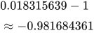 LaTeX:
0.018315639-1\approx-0.981684361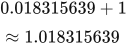 LaTeX:
0.018315639+1\approx1.018315639Step 4: divide.
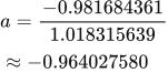 LaTeX:
a=\frac{-0.981684361}{1.018315639}\approx-0.964027580Step 5: square the activated output for its slope.
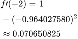 LaTeX:
f\prime(-2)=1-(-0.964027580)^2\approx0.070650825Final answer: a ≈ -0.964027580. Derivative ≈ 0.070650825.
tanh example 2
Question. For preactivation z = 0, calculate the tanh output and state its derivative.
Given
z = 0; activation = tanh.
To find
The output a and the derivative with respect to z.
Formula — which one and why
Use the activation named in the question. The derivative is a second calculation required for a backward pass.
z is the raw sum; a is the activated output; f′(z) is the local slope.
LaTeX: a=\frac{e^{2z}-1}{e^{2z}+1}LaTeX: f\prime(z)=1-a^2Yaad rakhne ka cue: Tanh ka answer −1 se 1; slope one minus output squared.
Solution — step by step
Step 1: double z before exponentiation.
 LaTeX:
2z=2(0)=0Step 2: calculate the exponential.
LaTeX: e^{0}\approx1.000000000Step 3: calculate numerator and denominator separately.
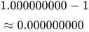 LaTeX:
1.000000000-1\approx0.000000000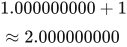 LaTeX:
1.000000000+1\approx2.000000000Step 4: divide.
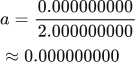 LaTeX:
a=\frac{0.000000000}{2.000000000}\approx0.000000000Step 5: square the activated output for its slope.
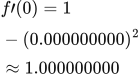 LaTeX:
f\prime(0)=1-(0.000000000)^2\approx1.000000000Final answer: a ≈ 0.000000000. Derivative ≈ 1.000000000.
tanh example 3
Question. For preactivation z = 2, calculate the tanh output and state its derivative.
Given
z = 2; activation = tanh.
To find
The output a and the derivative with respect to z.
Formula — which one and why
Use the activation named in the question. The derivative is a second calculation required for a backward pass.
z is the raw sum; a is the activated output; f′(z) is the local slope.
LaTeX: a=\frac{e^{2z}-1}{e^{2z}+1}LaTeX: f\prime(z)=1-a^2Yaad rakhne ka cue: Tanh ka answer −1 se 1; slope one minus output squared.
Solution — step by step
Step 1: double z before exponentiation.
 LaTeX:
2z=2(2)=4Step 2: calculate the exponential.
 LaTeX:
e^{4}\approx54.598150033Step 3: calculate numerator and denominator separately.
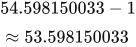 LaTeX:
54.598150033-1\approx53.598150033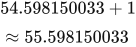 LaTeX:
54.598150033+1\approx55.598150033Step 4: divide.
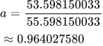 LaTeX:
a=\frac{53.598150033}{55.598150033}\approx0.964027580Step 5: square the activated output for its slope.
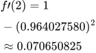 LaTeX:
f\prime(2)=1-(0.964027580)^2\approx0.070650825Final answer: a ≈ 0.964027580. Derivative ≈ 0.070650825.
ReLU and its derivative
ReLU compares its input with zero and keeps the larger value. Thus a negative input becomes zero and a positive input passes unchanged. Its slope is zero on the negative side and one on the positive side.
 LaTeX:
f(z)=\max(0,z)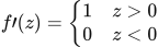 LaTeX:
f\prime(z)=\begin{cases}1&z>0\\0&z<0\end{cases}Drill 8 Activation contrast
Question
Question. For z = [−3,0,2], find ReLU and Leaky ReLU with α = 0.1, and the sigmoid derivative at z = 0.
Answer — step by step
Given
Inputs z = [−3,0,2].
Leaky-ReLU negative slope α = 0.1.
For the sigmoid derivative, use z = 0.
To find
Find ReLU and Leaky-ReLU outputs and the sigmoid slope at zero.
Formula — which one and why
ReLU and Leaky ReLU. ReLU returns zero for negative input and retains positive input. Leaky ReLU instead multiplies a negative input by its supplied slope.
z = preactivation; α (alpha) = supplied negative-side slope for Leaky ReLU. The derivative at zero needs an explicit convention.
LaTeX: \operatorname{ReLU}(z)=\max(0,z)LaTeX: \operatorname{LeakyReLU}(z)=\begin{cases}z&z\ge0\\\alpha z&z<0\end{cases}Yaad rakhne ka cue: Positive ko rehne do; negative ko zero. Leaky mein chhota negative rehne do.
Sigmoid and its slope. Use sigmoid when the neuron is specified to squash its preactivation into (0,1). Once its output is known, its derivative needs only output × (1−output).
z = preactivation; p = sigmoid output; e is the exponential base, not a prediction error in this formula.
LaTeX: p=\frac{1}{1+e^{-z}}LaTeX: \frac{dp}{dz}=p(1-p)Yaad rakhne ka cue: Sigmoid output p; uska slope p × (1−p).
Solution — step by step
Formulas and their meanings
ReLU compares the input with zero and returns the larger value.
LaTeX: \operatorname{ReLU}(z)=\max(0,z)Leaky ReLU uses the input unchanged when nonnegative, and multiplies it by α when negative.
LaTeX: \operatorname{LeakyReLU}(z)=\begin{cases}z&z\ge0\\\alpha z&z<0\end{cases}Step 1: apply ReLU separately to all three inputs
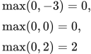 LaTeX:
\max(0,-3)=0,\quad \max(0,0)=0,\quad \max(0,2)=2ReLU output = [0, 0, 2].
Step 2: use α = 0.1 only on the negative input
 LaTeX:
0.1\times(-3)=-0.3The zero and positive entries remain 0 and 2. Leaky ReLU output = [−0.3, 0, 2].
Step 3: calculate sigmoid before its derivative
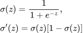 LaTeX:
\sigma(z)=\frac1{1+e^{-z}},\qquad \sigma'(z)=\sigma(z)[1-\sigma(z)]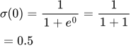 LaTeX:
\sigma(0)=\frac1{1+e^0}=\frac1{1+1}=0.5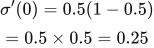 LaTeX:
\sigma'(0)=0.5(1-0.5)=0.5\times0.5=0.25The sigmoid value is 0.5 but its slope is 0.25. They are different quantities.
ReLU example 1
Question. For preactivation z = -2, calculate the ReLU output and state its derivative.
Given
z = -2; activation = ReLU.
To find
The output a and the derivative with respect to z.
Formula — which one and why
Use the activation named in the question. The derivative is a second calculation required for a backward pass.
z is the raw sum; a is the activated output; f′(z) is the local slope.
LaTeX: a=\max(0,z)Yaad rakhne ka cue: Positive side slope 1; negative side ReLU 0, Leaky α. Zero par convention likho.
Solution — step by step
Step 1: select the branch from the sign of z.
-2 is negative, so use the negative branch.
Step 2: calculate the output.
 LaTeX:
a=0Step 3: state the slope on that branch.
 LaTeX:
f\prime(-2)=0Final answer: a ≈ 0.000000000. Derivative ≈ 0.000000000.
ReLU example 2
Question. For preactivation z = 0, calculate the ReLU output and state its derivative.
Given
z = 0; activation = ReLU.
To find
The output a and the derivative with respect to z.
Formula — which one and why
Use the activation named in the question. The derivative is a second calculation required for a backward pass.
z is the raw sum; a is the activated output; f′(z) is the local slope.
LaTeX: a=\max(0,z)Yaad rakhne ka cue: Positive side slope 1; negative side ReLU 0, Leaky α. Zero par convention likho.
Solution — step by step
Step 1: select the branch from the sign of z.
Both branches meet at zero. The value is zero, but the left and right slopes differ.
Step 2: calculate the output.
LaTeX: a=0Step 3: state the slope on that branch.
The ordinary derivative at zero does not exist. A software subgradient convention may choose a value such as 0; state it if required.
Final answer: a ≈ 0.000000000. Ordinary derivative is undefined at zero.
ReLU example 3
Question. For preactivation z = 2, calculate the ReLU output and state its derivative.
Given
z = 2; activation = ReLU.
To find
The output a and the derivative with respect to z.
Formula — which one and why
Use the activation named in the question. The derivative is a second calculation required for a backward pass.
z is the raw sum; a is the activated output; f′(z) is the local slope.
LaTeX: a=\max(0,z)Yaad rakhne ka cue: Positive side slope 1; negative side ReLU 0, Leaky α. Zero par convention likho.
Solution — step by step
Step 1: select the branch from the sign of z.
2 is positive, so retain it.
Step 2: calculate the output.
 LaTeX:
a=2Step 3: state the slope on that branch.
 LaTeX:
f\prime(2)=1Final answer: a ≈ 2.000000000. Derivative ≈ 1.000000000.
Leaky ReLU
Leaky ReLU changes only the negative side: multiply a negative input by the small slope α. That negative sign remains. The value α is supplied by the question or chosen as a model setting; it is not the sigmoid function.
LaTeX: f(z)=\begin{cases}z&z\geq0\\az&z<0\end{cases}Drill 8 Activation contrast
Question
Question. For z = [−3,0,2], find ReLU and Leaky ReLU with α = 0.1, and the sigmoid derivative at z = 0.
Answer — step by step
Given
Inputs z = [−3,0,2].
Leaky-ReLU negative slope α = 0.1.
For the sigmoid derivative, use z = 0.
To find
Find ReLU and Leaky-ReLU outputs and the sigmoid slope at zero.
Formula — which one and why
ReLU and Leaky ReLU. ReLU returns zero for negative input and retains positive input. Leaky ReLU instead multiplies a negative input by its supplied slope.
z = preactivation; α (alpha) = supplied negative-side slope for Leaky ReLU. The derivative at zero needs an explicit convention.
LaTeX: \operatorname{ReLU}(z)=\max(0,z)LaTeX: \operatorname{LeakyReLU}(z)=\begin{cases}z&z\ge0\\\alpha z&z<0\end{cases}Yaad rakhne ka cue: Positive ko rehne do; negative ko zero. Leaky mein chhota negative rehne do.
Sigmoid and its slope. Use sigmoid when the neuron is specified to squash its preactivation into (0,1). Once its output is known, its derivative needs only output × (1−output).
z = preactivation; p = sigmoid output; e is the exponential base, not a prediction error in this formula.
LaTeX: p=\frac{1}{1+e^{-z}}LaTeX: \frac{dp}{dz}=p(1-p)Yaad rakhne ka cue: Sigmoid output p; uska slope p × (1−p).
Solution — step by step
Formulas and their meanings
ReLU compares the input with zero and returns the larger value.
LaTeX: \operatorname{ReLU}(z)=\max(0,z)Leaky ReLU uses the input unchanged when nonnegative, and multiplies it by α when negative.
LaTeX: \operatorname{LeakyReLU}(z)=\begin{cases}z&z\ge0\\\alpha z&z<0\end{cases}Step 1: apply ReLU separately to all three inputs
LaTeX: \max(0,-3)=0,\quad \max(0,0)=0,\quad \max(0,2)=2ReLU output = [0, 0, 2].
Step 2: use α = 0.1 only on the negative input
LaTeX: 0.1\times(-3)=-0.3The zero and positive entries remain 0 and 2. Leaky ReLU output = [−0.3, 0, 2].
Step 3: calculate sigmoid before its derivative
LaTeX: \sigma(z)=\frac1{1+e^{-z}},\qquad \sigma'(z)=\sigma(z)[1-\sigma(z)]LaTeX: \sigma(0)=\frac1{1+e^0}=\frac1{1+1}=0.5LaTeX: \sigma'(0)=0.5(1-0.5)=0.5\times0.5=0.25The sigmoid value is 0.5 but its slope is 0.25. They are different quantities.
Leaky ReLU example 1
Question. For preactivation z = -2, calculate the Leaky ReLU output and state its derivative. Use negative-side slope α = 0.1.
Given
z = -2; activation = Leaky ReLU.
α = 0.1.
To find
The output a and the derivative with respect to z.
Formula — which one and why
Use the activation named in the question. The derivative is a second calculation required for a backward pass.
z is the raw sum; a is the activated output; f′(z) is the local slope.
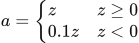 LaTeX:
a=\begin{cases}z&z\ge0\\0.1z&z<0\end{cases}Yaad rakhne ka cue: Positive side slope 1; negative side ReLU 0, Leaky α. Zero par convention likho.
Solution — step by step
Step 1: select the branch from the sign of z.
-2 is negative, so use the negative branch.
Step 2: calculate the output.
 LaTeX:
a=-0.2Step 3: state the slope on that branch.
 LaTeX:
f\prime(-2)=0.1Final answer: a ≈ -0.200000000. Derivative ≈ 0.100000000.
Leaky ReLU example 2
Question. For preactivation z = 0, calculate the Leaky ReLU output and state its derivative. Use negative-side slope α = 0.1.
Given
z = 0; activation = Leaky ReLU.
α = 0.1.
To find
The output a and the derivative with respect to z.
Formula — which one and why
Use the activation named in the question. The derivative is a second calculation required for a backward pass.
z is the raw sum; a is the activated output; f′(z) is the local slope.
LaTeX: a=\begin{cases}z&z\ge0\\0.1z&z<0\end{cases}Yaad rakhne ka cue: Positive side slope 1; negative side ReLU 0, Leaky α. Zero par convention likho.
Solution — step by step
Step 1: select the branch from the sign of z.
Both branches meet at zero. The value is zero, but the left and right slopes differ.
Step 2: calculate the output.
LaTeX: a=0Step 3: state the slope on that branch.
The ordinary derivative at zero does not exist. A software subgradient convention may choose a value such as 0; state it if required.
Final answer: a ≈ 0.000000000. Ordinary derivative is undefined at zero.
Leaky ReLU example 3
Question. For preactivation z = 2, calculate the Leaky ReLU output and state its derivative. Use negative-side slope α = 0.1.
Given
z = 2; activation = Leaky ReLU.
α = 0.1.
To find
The output a and the derivative with respect to z.
Formula — which one and why
Use the activation named in the question. The derivative is a second calculation required for a backward pass.
z is the raw sum; a is the activated output; f′(z) is the local slope.
LaTeX: a=\begin{cases}z&z\ge0\\0.1z&z<0\end{cases}Yaad rakhne ka cue: Positive side slope 1; negative side ReLU 0, Leaky α. Zero par convention likho.
Solution — step by step
Step 1: select the branch from the sign of z.
2 is positive, so retain it.
Step 2: calculate the output.
LaTeX: a=2Step 3: state the slope on that branch.
LaTeX: f\prime(2)=1Final answer: a ≈ 2.000000000. Derivative ≈ 1.000000000.
Stable softmax
Softmax turns several competing class scores into probabilities that add to one. Exponentiate each score, add those exponential values, and divide each one by their common total. Subtracting the same maximum score first gives the same probabilities with safer arithmetic.
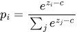 LaTeX:
p_i=\frac{e^{z_i-c}}{\sum_j e^{z_j-c}} LaTeX:
c=\max_j z_jDrill 9 Softmax and true class loss
Question
Question. Scores = [1,2,0], true one-hot class = [0,1,0]. Find probabilities and categorical cross-entropy.
Answer — step by step
Given
Logits = [1,2,0].
One-hot target = [0,1,0]: class 2 is correct.
To find
Find all three softmax probabilities and CCE.
Formula — which one and why
Stable softmax. Exponentiate each logit and divide by the sum. Subtracting the largest logit first keeps the exponentials numerically manageable and leaves the probabilities unchanged.
zⱼ = class j score; M = largest score; pⱼ = class j probability. All probabilities sum to 1.
 LaTeX:
M=\max_j z_j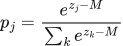 LaTeX:
p_j=\frac{e^{z_j-M}}{\sum_k e^{z_k-M}}Yaad rakhne ka cue: Largest score ghatao, exp nikalo, total se sabko divide karo.
Categorical cross-entropy. For mutually exclusive classes with a one-hot target, all zero-target terms disappear. The loss is the negative log of the probability assigned to the true class.
yⱼ = target entry; pⱼ = predicted probability; c = index of the true class. Use natural logarithms unless another base is specified.
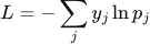 LaTeX:
L=-\sum_j y_j\ln p_j LaTeX:
L=-\ln p_cYaad rakhne ka cue: One-hot mein sirf correct class ki probability ka minus ln.
Solution — step by step
Meaning and formulas
The scores z are raw class scores. Softmax converts the whole group into class probabilities. The label [0,1,0] says class 2 is correct; it is not a set of predicted probabilities.
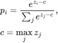 LaTeX:
p_i=\frac{e^{z_i-c}}{\sum_j e^{z_j-c}},\qquad c=\max_jz_jSubtracting the same c from every score keeps the probabilities unchanged and avoids very large exponentials.
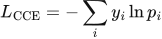 LaTeX:
L_{\mathrm{CCE}}=-\sum_i y_i\ln p_iStep 1: subtract the largest score
The largest of [1,2,0] is 2.
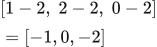 LaTeX:
[1-2,\;2-2,\;0-2]=[-1,0,-2]Step 2: calculate the three exponentials
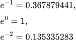 LaTeX:
e^{-1}=0.367879441,\quad e^0=1,\quad e^{-2}=0.135335283Step 3: add them to get one common denominator
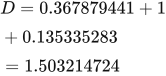 LaTeX:
D=0.367879441+1+0.135335283=1.503214724Step 4: divide each exponential by this denominator
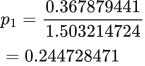 LaTeX:
p_1=\frac{0.367879441}{1.503214724}=0.244728471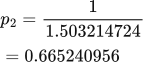 LaTeX:
p_2=\frac{1}{1.503214724}=0.665240956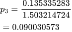 LaTeX:
p_3=\frac{0.135335283}{1.503214724}=0.090030573The probabilities add to 1, apart from rounding. Class 2 has the highest score and the highest probability.
Step 5: use the probability of the correct class in CCE
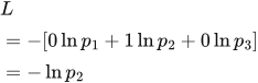 LaTeX:
L=-[0\ln p_1+1\ln p_2+0\ln p_3]=-\ln p_2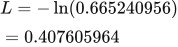 LaTeX:
L=-\ln(0.665240956)=0.407605964Final answer: probabilities ≈ [0.244728, 0.665241, 0.090031]; CCE ≈ 0.407606.
Softmax for [0, 0, 0]
Question. Find stable softmax probabilities for logits [0, 0, 0].
Given
Logits = [0, 0, 0]; there are three mutually exclusive classes.
To find
All three class probabilities.
Formula — which one and why
Subtracting one common maximum preserves probabilities and keeps exponentials well scaled. Normalize using one shared sum.
A logit is a raw class score. c is the largest score; pᵢ is probability for class i.
LaTeX: c=\max_j z_jLaTeX: p_i=\frac{e^{z_i-c}}{\sum_j e^{z_j-c}}Yaad rakhne ka cue: Max minus, e-power, same denominator se sab divide.
Solution — step by step
Step 1: subtract the largest score from every entry.
 LaTeX:
z-c=\begin{bmatrix}0&0&0\end{bmatrix}Step 2: exponentiate shifted entry 1.
LaTeX: e^{0}\approx1.000000000Step 3: exponentiate shifted entry 2.
LaTeX: e^{0}\approx1.000000000Step 4: exponentiate shifted entry 3.
LaTeX: e^{0}\approx1.000000000Step 5: add all exponentials into one denominator.
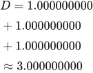 LaTeX:
D=1.000000000+1.000000000+1.000000000\approx3.000000000Step 6: divide entry 1 by the same denominator.
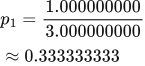 LaTeX:
p_1=\frac{1.000000000}{3.000000000}\approx0.333333333Step 7: divide entry 2 by the same denominator.
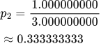 LaTeX:
p_2=\frac{1.000000000}{3.000000000}\approx0.333333333Step 8: divide entry 3 by the same denominator.
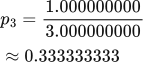 LaTeX:
p_3=\frac{1.000000000}{3.000000000}\approx0.333333333Final answer: Probabilities ≈ [0.333333333, 0.333333333, 0.333333333]; they sum to 1 within rounding.
Softmax for [1, 2, 3]
Question. Find stable softmax probabilities for logits [1, 2, 3].
Given
Logits = [1, 2, 3]; there are three mutually exclusive classes.
To find
All three class probabilities.
Formula — which one and why
Subtracting one common maximum preserves probabilities and keeps exponentials well scaled. Normalize using one shared sum.
A logit is a raw class score. c is the largest score; pᵢ is probability for class i.
LaTeX: c=\max_j z_jLaTeX: p_i=\frac{e^{z_i-c}}{\sum_j e^{z_j-c}}Yaad rakhne ka cue: Max minus, e-power, same denominator se sab divide.
Solution — step by step
Step 1: subtract the largest score from every entry.
 LaTeX:
z-c=\begin{bmatrix}-2&-1&0\end{bmatrix}Step 2: exponentiate shifted entry 1.
LaTeX: e^{-2}\approx0.135335283Step 3: exponentiate shifted entry 2.
 LaTeX:
e^{-1}\approx0.367879441Step 4: exponentiate shifted entry 3.
LaTeX: e^{0}\approx1.000000000Step 5: add all exponentials into one denominator.
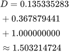 LaTeX:
D=0.135335283+0.367879441+1.000000000\approx1.503214724Step 6: divide entry 1 by the same denominator.
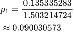 LaTeX:
p_1=\frac{0.135335283}{1.503214724}\approx0.090030573Step 7: divide entry 2 by the same denominator.
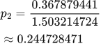 LaTeX:
p_2=\frac{0.367879441}{1.503214724}\approx0.244728471Step 8: divide entry 3 by the same denominator.
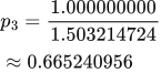 LaTeX:
p_3=\frac{1.000000000}{1.503214724}\approx0.665240956Final answer: Probabilities ≈ [0.090030573, 0.244728471, 0.665240956]; they sum to 1 within rounding.
Squared and absolute losses
SSE, half SSE and MSE start with the same errors but apply different final divisions. First understand what an error and its square mean. The full question below keeps all three answers separate.
LaTeX: \mathrm{SSE}=\sum_i(o_i-y_i)^2LaTeX: L_{\mathrm{half}}=\frac{\mathrm{SSE}}2LaTeX: L_{\mathrm{MSE}}=\frac{\mathrm{SSE}}nLaTeX: L_{\mathrm{MAE}}=\frac1n\sum_i|o_i-y_i|Loss: how one wrong prediction becomes a number
Definition. A residual is the signed prediction error. Squared-error objectives aggregate squared residuals; their scaling convention changes both the reported loss and its derivative.
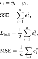 LaTeX:
e_i=\hat y_i-y_i,\qquad \mathrm{SSE}=\sum_{i=1}^{n}e_i^2,\qquad L_{\mathrm{half}}=\frac12\sum_{i=1}^{n}e_i^2,\qquad \mathrm{MSE}=\frac1n\sum_{i=1}^{n}e_i^2For this definition of n, each i indexes one included scalar prediction. In a multi-output batch, state whether the mean is over examples, output coordinates, or both. Half SSE and MSE happen to agree when n = 2; they are not generally the same objective.
Derivatives and their scaling
When differentiating with respect to prediction j, all other prediction terms are constant. The derivative of the j-th square is twice its residual:
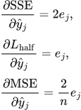 LaTeX:
\frac{\partial\mathrm{SSE}}{\partial\hat y_j}=2e_j,\qquad \frac{\partial L_{\mathrm{half}}}{\partial\hat y_j}=e_j,\qquad \frac{\partial\mathrm{MSE}}{\partial\hat y_j}=\frac{2}{n}e_jThe factor 1/2 cancels the derivative's factor 2. The factor 1/n instead produces 2/n. A weight derivative must also multiply by the derivative of the prediction with respect to that weight.
Question. Predictions are [0.2, 0.7, 0.4] and targets are [0, 1, 1]. Find SSE, half SSE and MSE, then their gradients with respect to the prediction vector.
Given
Predictions = [0.2,0.7,0.4].
Targets = [0,1,1]; n = 3 scalar predictions.
To find
Find SSE, half SSE and MSE, then all three prediction-gradient lists.
Formula — which one and why
Squared-error objectives. Calculate signed errors first and square them. SSE adds the squares; half SSE divides that sum by 2; MSE divides by the number of scalar predictions. These denominators are different conventions.
ŷᵢ = prediction; yᵢ = target; eᵢ = signed error; n = number of scalar predictions included in the stated loss.
 LaTeX:
e_i=\hat y_i-y_i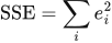 LaTeX:
\mathrm{SSE}=\sum_i e_i^2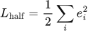 LaTeX:
L_{\mathrm{half}}=\frac12\sum_i e_i^2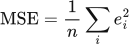 LaTeX:
\mathrm{MSE}=\frac1n\sum_i e_i^2Yaad rakhne ka cue: Pehle error square; phir question ke hisaab se sum, half ya mean.
Solution — step by step
Step 1: calculate the three signed prediction errors.
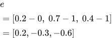 LaTeX:
e=[0.2-0,\ 0.7-1,\ 0.4-1]=[0.2,-0.3,-0.6]Step 2: square every error.
 LaTeX:
e\odot e=[0.04,0.09,0.36]Step 3: add the three squared errors.
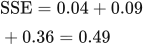 LaTeX:
\mathrm{SSE}=0.04+0.09+0.36=0.49Step 4: apply the requested loss divisors.
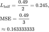 LaTeX:
L_{\mathrm{half}}=\frac{0.49}{2}=0.245,\qquad \mathrm{MSE}=\frac{0.49}{3}\approx0.163333333Step 5: multiply every error by 2 for the SSE gradient.
 LaTeX:
\nabla_{\hat y}\mathrm{SSE}=[0.4,-0.6,-1.2]Step 6: use each error itself for the half-SSE gradient.
 LaTeX:
\nabla_{\hat y}L_{\mathrm{half}}=[0.2,-0.3,-0.6]Step 7: multiply every error by 2/3 for the MSE gradient.
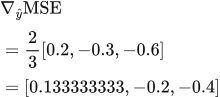 LaTeX:
\nabla_{\hat y}\mathrm{MSE}=\frac23[0.2,-0.3,-0.6]=[0.133333333,-0.2,-0.4]The residual signs survive in the gradients even though the losses are nonnegative. Multiplying a loss by a positive constant leaves its unregularized minimizers unchanged, but scales its gradients and therefore its updates at a fixed learning rate.
Drill 2 Half sum versus mean
Question
Question. Predictions = [0.2,0.7,0.4], targets = [0,1,1]. Find SSE, half SSE and MSE.
Answer — step by step
Given
Predictions = [0.2, 0.7, 0.4].
Targets = [0, 1, 1]; number of outputs n = 3.
To find
Find SSE, half SSE, MSE and the prediction gradients requested in the question.
Formula — which one and why
Squared-error objectives. Calculate signed errors first and square them. SSE adds the squares; half SSE divides that sum by 2; MSE divides by the number of scalar predictions. These denominators are different conventions.
ŷᵢ = prediction; yᵢ = target; eᵢ = signed error; n = number of scalar predictions included in the stated loss.
LaTeX: e_i=\hat y_i-y_iLaTeX: \mathrm{SSE}=\sum_i e_i^2LaTeX: L_{\mathrm{half}}=\frac12\sum_i e_i^2LaTeX: \mathrm{MSE}=\frac1n\sum_i e_i^2Yaad rakhne ka cue: Pehle error square; phir question ke hisaab se sum, half ya mean.
Solution — step by step
Given values and loss definitions
There are n = 3 prediction–target pairs. Use the supplied predictions directly; no rounding to class labels is required. Let eᵢ = ŷᵢ − yᵢ be the signed residual for pair i.
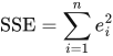 LaTeX:
\mathrm{SSE}=\sum_{i=1}^{n}e_i^2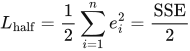 LaTeX:
L_{\mathrm{half}}=\frac12\sum_{i=1}^{n}e_i^2=\frac{\mathrm{SSE}}2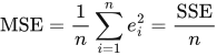 LaTeX:
\mathrm{MSE}=\frac1n\sum_{i=1}^{n}e_i^2=\frac{\mathrm{SSE}}nSSE is the sum of squared errors. Half SSE and MSE rescale that same sum by different denominators: 2 and n, respectively.
Step 1: calculate each residual and its square
| Pair | Prediction ŷᵢ | Target yᵢ | Residual ŷᵢ − yᵢ | Squared residual |
|---|---|---|---|---|
| 1 | 0.2 | 0 | 0.2 − 0 = 0.2 | (0.2)² = 0.04 |
| 2 | 0.7 | 1 | 0.7 − 1 = −0.3 | (−0.3)² = 0.09 |
| 3 | 0.4 | 1 | 0.4 − 1 = −0.6 | (−0.6)² = 0.36 |
Step 2: sum the squared residuals
LaTeX: \mathrm{SSE}=0.04+0.09+0.36=0.49Square each residual before summing. Squaring the sum of signed residuals would be a different quantity, because positive and negative residuals could cancel.
Step 3: apply each requested normalization
For half SSE, the denominator is 2:
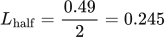 LaTeX:
L_{\mathrm{half}}=\frac{0.49}{2}=0.245For MSE, the denominator is the number of pairs, n = 3:
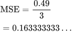 LaTeX:
\mathrm{MSE}=\frac{0.49}{3}=0.163333333\ldotsFinal answer: SSE = 0.49; half SSE = 0.245; MSE ≈ 0.163333. They represent the same residuals at different scales. Half SSE and MSE coincide when n = 2; they do not coincide for these three nonzero residuals. No derivative is required by this question.
Absolute error uses a different operation
Question. Targets are [2, 4] and predictions are [1, 6]. Find mean absolute error.
Given
Targets = [2,4]; predictions = [1,6]; n = 2.
To find
Find mean absolute error.
Formula — which one and why
Mean absolute error. Absolute value removes the sign of each prediction error without squaring its magnitude. Average those magnitudes.
n = number of predictions. |e| means the nonnegative magnitude of error e.
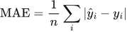 LaTeX:
\mathrm{MAE}=\frac1n\sum_i|\hat y_i-y_i|Yaad rakhne ka cue: MAE mein magnitude; MSE mein square.
Solution — step by step
The signed errors are 1 − 2 = −1 and 6 − 4 = 2. Absolute value keeps the size of a number without its sign, so their absolute errors are 1 and 2. Add them to obtain 3. There are two prediction–target pairs, so divide by 2.
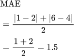 LaTeX:
\mathrm{MAE}=\frac{|1-2|+|6-4|}{2}=\frac{1+2}{2}=1.5Final answer: MAE = 1.5. Do not square the errors for MAE.
Binary cross entropy
Binary cross-entropy measures how much probability was assigned to the correct binary answer. A target of 1 keeps the −ln(p) term; a target of 0 keeps the −ln(1−p) term. The factors y and 1−y select the appropriate term.
LaTeX: L=-[y\ln p+(1-y)\ln(1-p)]Drill 7 Sigmoid with binary cross entropy
Question
Question. A binary classifier has logit z = 1, target 1. Find probability, BCE and the gradient with respect to z.
Answer — step by step
Given
Logit z = 1; binary target y = 1.
Output: sigmoid; loss: binary cross-entropy.
To find
Find probability, BCE and the loss derivative with respect to z.
Formula — which one and why
Sigmoid and its slope. Use sigmoid when the neuron is specified to squash its preactivation into (0,1). Once its output is known, its derivative needs only output × (1−output).
z = preactivation; p = sigmoid output; e is the exponential base, not a prediction error in this formula.
LaTeX: p=\frac{1}{1+e^{-z}}LaTeX: \frac{dp}{dz}=p(1-p)Yaad rakhne ka cue: Sigmoid output p; uska slope p × (1−p).
Binary cross-entropy. For a binary target, choose the probability of the correct outcome and take its negative natural log. Sigmoid plus BCE has combined logit derivative p−y.
y is 0 or 1; p is the predicted probability of class 1; z is the sigmoid logit. The p−y derivative already includes the sigmoid derivative.
LaTeX: L=-[y\ln p+(1-y)\ln(1-p)] LaTeX:
\frac{\partial L}{\partial z}=p-yYaad rakhne ka cue: Binary target 1 ho toh −ln(p); target 0 ho toh −ln(1−p).
Solution — step by step
Meaning and formulas
A logit is the raw score before sigmoid. Sigmoid converts it to a probability p. The target y = 1 says the positive class is correct. Binary cross-entropy measures how little probability the model assigned to the correct binary outcome.
 LaTeX:
p=\frac1{1+e^{-z}} LaTeX:
L=-\left[y\ln p+(1-y)\ln(1-p)\right]For sigmoid combined with this loss, the gradient with respect to the logit has the simplified form:
LaTeX: \frac{\partial L}{\partial z}=p-yStep 1: convert logit 1 into probability
LaTeX: e^{-1}\approx0.367879441 LaTeX:
1+e^{-1}\approx1.367879441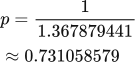 LaTeX:
p=\frac1{1.367879441}\approx0.731058579Step 2: substitute the target in the full loss formula
 LaTeX:
L=-\left[1\ln(0.731058579)+(1-1)\ln(1-0.731058579)\right]The second term has multiplier zero, so it contributes zero.
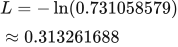 LaTeX:
L=-\ln(0.731058579)\approx0.313261688Step 3: calculate the combined gradient
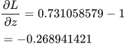 LaTeX:
\frac{\partial L}{\partial z}=0.731058579-1=-0.268941421Final answer: probability ≈ 0.731059; BCE ≈ 0.313262; logit gradient ≈ −0.268941. The simplified gradient already includes sigmoid's effect. Multiplying by sigmoid's slope again would apply it twice.
Binary cross-entropy: target 1, predicted positive-class probability 0.8
Question. A binary classifier predicts P(y=1) = 0.8. The target is y = 1. Calculate binary cross-entropy using natural logarithms.
Given
Target y = 1; p = P(y=1) = 0.8; use natural log ln.
To find
The binary cross-entropy loss for this one example.
Formula — which one and why
The target selects the probability assigned to the correct class. Take its negative natural logarithm.
p is always the probability of class 1. When y = 0, the correct-class probability is 1−p.
LaTeX: L=-[y\ln p+(1-y)\ln(1-p)]Yaad rakhne ka cue: True class ki probability lo, uska minus ln lo.
Solution — step by step
Step 1: identify the correct-class probability.
 LaTeX:
p=0.8Step 2: evaluate its natural logarithm.
 LaTeX:
\ln(0.8)\approx-0.223143551Step 3: apply the minus sign outside the logarithm.
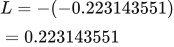 LaTeX:
L=-(-0.223143551)=0.223143551Final answer: Loss ≈ 0.223143551 nats.
Binary cross-entropy: target 0, predicted positive-class probability 0.8
Question. A binary classifier predicts P(y=1) = 0.8. The target is y = 0. Calculate binary cross-entropy using natural logarithms.
Given
Target y = 0; p = P(y=1) = 0.8; use natural log ln.
To find
The binary cross-entropy loss for this one example.
Formula — which one and why
The target selects the probability assigned to the correct class. Take its negative natural logarithm.
p is always the probability of class 1. When y = 0, the correct-class probability is 1−p.
LaTeX: L=-[y\ln p+(1-y)\ln(1-p)]Yaad rakhne ka cue: True class ki probability lo, uska minus ln lo.
Solution — step by step
Step 1: identify the correct-class probability.
 LaTeX:
1-p=1-0.8=0.2Step 2: evaluate its natural logarithm.
 LaTeX:
\ln(0.2)\approx-1.609437912Step 3: apply the minus sign outside the logarithm.
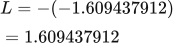 LaTeX:
L=-(-1.609437912)=1.609437912Final answer: Loss ≈ 1.609437912 nats.
Binary cross-entropy: target 1, predicted positive-class probability 0.5
Question. A binary classifier predicts P(y=1) = 0.5. The target is y = 1. Calculate binary cross-entropy using natural logarithms.
Given
Target y = 1; p = P(y=1) = 0.5; use natural log ln.
To find
The binary cross-entropy loss for this one example.
Formula — which one and why
The target selects the probability assigned to the correct class. Take its negative natural logarithm.
p is always the probability of class 1. When y = 0, the correct-class probability is 1−p.
LaTeX: L=-[y\ln p+(1-y)\ln(1-p)]Yaad rakhne ka cue: True class ki probability lo, uska minus ln lo.
Solution — step by step
Step 1: identify the correct-class probability.
 LaTeX:
p=0.5Step 2: evaluate its natural logarithm.
 LaTeX:
\ln(0.5)\approx-0.693147181Step 3: apply the minus sign outside the logarithm.
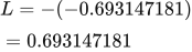 LaTeX:
L=-(-0.693147181)=0.693147181Final answer: Loss ≈ 0.693147181 nats.
Categorical cross entropy
For one-hot multiclass targets, only one target entry is 1. The other entries are zero, so the loss becomes minus the logarithm of the true class probability. The worked question first calculates every softmax probability, then selects the correct one.
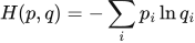 LaTeX:
H(p,q)=-\sum_i p_i\ln q_i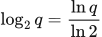 LaTeX:
\log_2q=\frac{\ln q}{\ln2}LaTeX: L=-\sum_i y_i\ln p_i=-\ln p_{true}Cross-entropy for probability distributions
Definition. For a discrete target distribution p and a predicted distribution q over the same classes, cross-entropy is the target-weighted negative logarithm of the predicted probabilities.
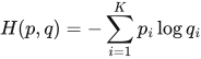 LaTeX:
H(p,q)=-\sum_{i=1}^{K}p_i\log q_iHere pᵢ and qᵢ refer to the same class i, and each distribution sums to 1. The target supplies the weights outside the logarithm; the prediction goes inside it. If the target is one-hot, only the correct-class term remains. For a soft target with several nonzero entries, include all its nonzero terms.
Logarithm base and units
Natural logarithms produce nats; base-2 logarithms produce bits. These notes use ln unless a question states another base. On a calculator with ln, use the change-of-base rule for base 2:
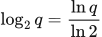 LaTeX:
\log_2 q=\frac{\ln q}{\ln 2}For a target entry pᵢ = 0, its contribution is defined as zero. If pᵢ > 0 but qᵢ = 0, the loss is infinite. For numerical stability, software normally calculates cross-entropy from logits or carefully handles boundary probabilities.
A target distribution with two nonzero entries
Question. A two-class target distribution is p = [0.75, 0.25] and the model predicts q = [0.5, 0.5]. Calculate cross-entropy using natural logarithms and using base-2 logarithms.
Given
A two-class target distribution is p = [0.75, 0.25] and the model predicts q = [0.5, 0.5].
Calculate cross-entropy using natural logarithms and using base-2 logarithms.
To find
Find cross-entropy in the requested units.
Formula — which one and why
Cross-entropy between distributions. Weight each negative log prediction by the target probability. Unlike one-hot targets, several terms can contribute.
pᵢ = target-distribution probability; qᵢ = predicted probability. Natural logs give nats; base-2 logs give bits.
LaTeX: H(p,q)=-\sum_i p_i\ln q_i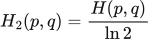 LaTeX:
H_2(p,q)=\frac{H(p,q)}{\ln2}Yaad rakhne ka cue: Target probability batati hai kis log-loss ka kitna hissa lena hai.
Solution — step by step
Step 1: write the two terms. Both target entries are nonzero, so neither term can be discarded.
 LaTeX:
H(p,q)=-[0.75\ln(0.5)+0.25\ln(0.5)]Step 2: calculate the logarithms.
LaTeX: \ln(0.5)\approx-0.693147181Step 3: weight each negative logarithm by its target probability.
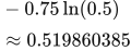 LaTeX:
-0.75\ln(0.5)\approx0.519860385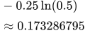 LaTeX:
-0.25\ln(0.5)\approx0.173286795Step 4: add the contributions, retaining calculator precision.
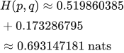 LaTeX:
H(p,q)\approx0.519860385+0.173286795\approx0.693147181\ \text{nats}Step 5: repeat with base 2. Since 2⁻¹ = 0.5, log₂(0.5) = −1.
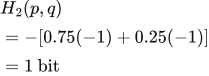 LaTeX:
H_2(p,q)=-[0.75(-1)+0.25(-1)]=1\ \text{bit}Final answer: 0.693147 nats or 1 bit. The distributions are unchanged; the logarithm base changes the unit and the numerical scale.
Cross-entropy, entropy and relative entropy
These names are related but do not denote the same quantity. Entropy uses the target distribution in both positions. Relative entropy, also called KL divergence, measures their difference through a probability ratio.
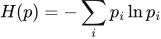 LaTeX:
H(p)=-\sum_i p_i\ln p_i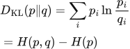 LaTeX:
D_{\mathrm{KL}}(p\Vert q)=\sum_i p_i\ln\frac{p_i}{q_i}=H(p,q)-H(p)For fixed p, H(p) is constant with respect to the model parameters, so minimizing cross-entropy also minimizes this KL divergence. KL is clarified here to distinguish the terminology; it is not a separately named unit in the official syllabus.
Question. For the same p = [0.75, 0.25] and q = [0.5, 0.5], find H(p) and DKL(p ∥ q) in nats.
Given
For the same p = [0.75, 0.25] and q = [0.5, 0.5], find H(p) and DKL(p ∥ q) in nats.
To find
Find entropy and KL divergence in nats.
Formula — which one and why
Entropy and relative entropy. Entropy measures the target distribution’s uncertainty. Relative entropy measures the extra cross-entropy when q is used instead of p.
p = target distribution; q = model distribution; H(p) = entropy; DKL = Kullback–Leibler divergence.
LaTeX: H(p)=-\sum_i p_i\ln p_i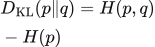 LaTeX:
D_{\mathrm{KL}}(p\Vert q)=H(p,q)-H(p)Yaad rakhne ka cue: KL = cross-entropy minus target ki own entropy.
Solution — step by step
Step 1: calculate the target entropy.
 LaTeX:
H(p)=-[0.75\ln(0.75)+0.25\ln(0.25)]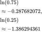 LaTeX:
\ln(0.75)\approx-0.287682072,\qquad\ln(0.25)\approx-1.386294361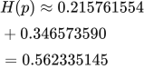 LaTeX:
H(p)\approx0.215761554+0.346573590=0.562335145Step 2: subtract target entropy from cross-entropy.
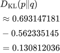 LaTeX:
D_{\mathrm{KL}}(p\Vert q)\approx0.693147181-0.562335145=0.130812036Final answer: H(p) ≈ 0.562335 nats and DKL(p ∥ q) ≈ 0.130812 nats. For a one-hot target H(p) = 0, so cross-entropy and this KL divergence coincide; for this soft target they differ.
Drill 9 Softmax and true class loss
Question
Question. Scores = [1,2,0], true one-hot class = [0,1,0]. Find probabilities and categorical cross-entropy.
Answer — step by step
Given
Logits = [1,2,0].
One-hot target = [0,1,0]: class 2 is correct.
To find
Find all three softmax probabilities and CCE.
Formula — which one and why
Stable softmax. Exponentiate each logit and divide by the sum. Subtracting the largest logit first keeps the exponentials numerically manageable and leaves the probabilities unchanged.
zⱼ = class j score; M = largest score; pⱼ = class j probability. All probabilities sum to 1.
LaTeX: M=\max_j z_jLaTeX: p_j=\frac{e^{z_j-M}}{\sum_k e^{z_k-M}}Yaad rakhne ka cue: Largest score ghatao, exp nikalo, total se sabko divide karo.
Categorical cross-entropy. For mutually exclusive classes with a one-hot target, all zero-target terms disappear. The loss is the negative log of the probability assigned to the true class.
yⱼ = target entry; pⱼ = predicted probability; c = index of the true class. Use natural logarithms unless another base is specified.
LaTeX: L=-\sum_j y_j\ln p_jLaTeX: L=-\ln p_cYaad rakhne ka cue: One-hot mein sirf correct class ki probability ka minus ln.
Solution — step by step
Meaning and formulas
The scores z are raw class scores. Softmax converts the whole group into class probabilities. The label [0,1,0] says class 2 is correct; it is not a set of predicted probabilities.
LaTeX: p_i=\frac{e^{z_i-c}}{\sum_j e^{z_j-c}},\qquad c=\max_jz_jSubtracting the same c from every score keeps the probabilities unchanged and avoids very large exponentials.
LaTeX: L_{\mathrm{CCE}}=-\sum_i y_i\ln p_iStep 1: subtract the largest score
The largest of [1,2,0] is 2.
LaTeX: [1-2,\;2-2,\;0-2]=[-1,0,-2]Step 2: calculate the three exponentials
LaTeX: e^{-1}=0.367879441,\quad e^0=1,\quad e^{-2}=0.135335283Step 3: add them to get one common denominator
LaTeX: D=0.367879441+1+0.135335283=1.503214724Step 4: divide each exponential by this denominator
LaTeX: p_1=\frac{0.367879441}{1.503214724}=0.244728471LaTeX: p_2=\frac{1}{1.503214724}=0.665240956LaTeX: p_3=\frac{0.135335283}{1.503214724}=0.090030573The probabilities add to 1, apart from rounding. Class 2 has the highest score and the highest probability.
Step 5: use the probability of the correct class in CCE
LaTeX: L=-[0\ln p_1+1\ln p_2+0\ln p_3]=-\ln p_2LaTeX: L=-\ln(0.665240956)=0.407605964Final answer: probabilities ≈ [0.244728, 0.665241, 0.090031]; CCE ≈ 0.407606.
Output delta for half squared loss
Delta is a short name for the loss derivative with respect to a neuron’s raw input z. For half squared loss, multiply prediction minus target by the activation’s derivative. The result is then multiplied by an incoming activation to obtain a weight gradient.
LaTeX: \delta^{out}=(o-y)f\prime(z)Loss scaling: derive the gradient instead of guessing a factor
1. One error, three possible objectives
Let a be a prediction and y a fixed target. The error is a − y. The derivative of that error with respect to a is 1 because y stays fixed. Apply the chain rule to its square:
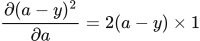 LaTeX:
\frac{\partial (a-y)^2}{\partial a}=2(a-y)\times1Multiplying the objective by a constant multiplies its derivative by the same constant. This gives the common loss conventions below.
| Stated loss over n outputs | Derivative with respect to one prediction aⱼ |
|---|---|
| SSE: sum of all squared errors | 2(aⱼ − yⱼ) |
| Half SSE: half of that sum | aⱼ − yⱼ |
| MSE: that sum divided by n | 2(aⱼ − yⱼ)/n |
| Half MSE: that sum divided by 2n | (aⱼ − yⱼ)/n |
2. Why only the matching output appears
Suppose three predictions are separate output variables a₁, a₂ and a₃. When differentiating the loss with respect to a₂, the a₁ and a₃ terms are constant with respect to that output variable, so their direct derivatives are zero. The remaining term is the error of output 2, with the correct scaling factor.
Later, a shared hidden weight may influence all three predictions. Backpropagation then combines those separate output contributions through the chain rule. “Differentiate with respect to one output” and “differentiate with respect to a shared weight” are different stages.
3. The activation contributes another factor
If a = sigmoid(z), the derivative of a with respect to its input is a(1 − a). For half SSE, the output delta is therefore:
 LaTeX:
\delta=\frac{\partial L}{\partial z}=(a-y)a(1-a)For a linear output, the activation derivative is 1. For positive ReLU input it is also 1; for negative ReLU input it is 0. Always use the derivative of the activation actually given in the question.
4. A numerical comparison
For a = 0.7 and y = 1, the signed error is −0.3. For half SSE with sigmoid, the activation derivative is 0.7 × 0.3 = 0.21. The output delta is −0.3 × 0.21 = −0.063. With plain SSE it doubles to −0.126. With MSE over three outputs it is −0.126/3 = −0.042.
The forward prediction 0.7 did not change. The loss convention changed the gradient scale. This is why the first line of a backpropagation answer should state the loss being used.
Complete sigmoid training example
Question. A sigmoid neuron has input 2, weight 0, bias 0, target 1 and half squared loss. Will gradient descent increase or decrease the weight? Use learning rate 0.1 and calculate the exact update.
Given
x = 2; w = 0; b = 0; y = 1.
Sigmoid output; half squared loss; η = 0.1.
To find
Find the weight-gradient sign, exact weight update and resulting weight.
Formula — which one and why
Weighted sum and activation. Each input is multiplied by its connection weight. Add these contributions, add the bias once, then apply the stated activation.
xᵢ = input i; wᵢ = its weight; b = bias; z = sum before activation; a = output after activation; f = the specified activation function.
LaTeX: z=\sum_iw_ix_i+bLaTeX: a=f(z)Yaad rakhne ka cue: Input × weight, sabka sum, bias once, phir activation.
Sigmoid and its slope. Use sigmoid when the neuron is specified to squash its preactivation into (0,1). Once its output is known, its derivative needs only output × (1−output).
z = preactivation; p = sigmoid output; e is the exponential base, not a prediction error in this formula.
LaTeX: p=\frac{1}{1+e^{-z}}LaTeX: \frac{dp}{dz}=p(1-p)Yaad rakhne ka cue: Sigmoid output p; uska slope p × (1−p).
Half summed squared loss. This loss convention takes one-half of the sum of squared prediction errors. Use it when the question specifies it, or explicitly state it as an assumption when the paper omits the loss. Differentiating cancels the factor one-half against the square derivative.
oⱼ = output j; yⱼ = target j; L = half summed squared loss under the stated or explicitly assumed convention.
LaTeX: L=\frac12\sum_j(o_j-y_j)^2LaTeX: \frac{\partial L}{\partial o_j}=o_j-y_jYaad rakhne ka cue: Half aur square ka 2 cancel: output derivative = prediction − target.
Backpropagation. The loss tells us how each output must change. Multiply by that neuron’s activation slope to obtain its delta. A weight gradient is receiving delta × sending value. Hidden deltas must include every outgoing path.
δ (delta) = derivative of loss with respect to a neuron’s preactivation; f′ = activation derivative; aᵢ = sending activation; Wⱼᵢ = connection weight. Use the exact loss scaling in the question.
LaTeX: \delta_{o_j}=\frac{\partial L}{\partial o_j}f_o\prime(z_{o_j})LaTeX: \delta_{h_i}=f_h\prime(z_{h_i})\sum_jW_{ji}^{(2)}\delta_{o_j}LaTeX: \frac{\partial L}{\partial W_{ji}}=\delta_ja_iLaTeX: \frac{\partial L}{\partial b_j}=\delta_jLaTeX: W_{ji,\mathrm{new}}=W_{ji}-\eta\frac{\partial L}{\partial W_{ji}}Yaad rakhne ka cue: Receiving delta × sending value = us connection ka gradient.
Solution — step by step
Step 1 forward: net = 0(2) + 0 = 0; sigmoid output = 0.5.
Step 2 backward: prediction minus target = 0.5 − 1 = −0.5. Sigmoid slope = 0.5(1 − 0.5) = 0.25. Delta = −0.5 × 0.25 = −0.125.
Step 3 gradients and update: weight gradient = −0.125 × 2 = −0.25. New weight = 0 − 0.1(−0.25) = 0.025. Bias gradient = −0.125; new bias = 0.0125. Both increase. With positive input, these changes initially raise the prediction toward the target. Your intuition and arithmetic now agree.
Drill 10 Sigmoid neuron gradient
Question
Question. x = 2, w = 0.5, b = 0, y = 1, half squared loss, η = 0.1. Find one weight and bias update.
Answer — step by step
Given
x = 2; w = 0.5; b = 0; target y = 1.
Activation: sigmoid; loss: half squared error.
Learning rate η = 0.1.
To find
Find the output, delta, weight/bias gradients and one update.
Formula — which one and why
Weighted sum and activation. Each input is multiplied by its connection weight. Add these contributions, add the bias once, then apply the stated activation.
xᵢ = input i; wᵢ = its weight; b = bias; z = sum before activation; a = output after activation; f = the specified activation function.
LaTeX: z=\sum_iw_ix_i+bLaTeX: a=f(z)Yaad rakhne ka cue: Input × weight, sabka sum, bias once, phir activation.
Sigmoid and its slope. Use sigmoid when the neuron is specified to squash its preactivation into (0,1). Once its output is known, its derivative needs only output × (1−output).
z = preactivation; p = sigmoid output; e is the exponential base, not a prediction error in this formula.
LaTeX: p=\frac{1}{1+e^{-z}}LaTeX: \frac{dp}{dz}=p(1-p)Yaad rakhne ka cue: Sigmoid output p; uska slope p × (1−p).
Half summed squared loss. This loss convention takes one-half of the sum of squared prediction errors. Use it when the question specifies it, or explicitly state it as an assumption when the paper omits the loss. Differentiating cancels the factor one-half against the square derivative.
oⱼ = output j; yⱼ = target j; L = half summed squared loss under the stated or explicitly assumed convention.
LaTeX: L=\frac12\sum_j(o_j-y_j)^2LaTeX: \frac{\partial L}{\partial o_j}=o_j-y_jYaad rakhne ka cue: Half aur square ka 2 cancel: output derivative = prediction − target.
Backpropagation. The loss tells us how each output must change. Multiply by that neuron’s activation slope to obtain its delta. A weight gradient is receiving delta × sending value. Hidden deltas must include every outgoing path.
δ (delta) = derivative of loss with respect to a neuron’s preactivation; f′ = activation derivative; aᵢ = sending activation; Wⱼᵢ = connection weight. Use the exact loss scaling in the question.
LaTeX: \delta_{o_j}=\frac{\partial L}{\partial o_j}f_o\prime(z_{o_j})LaTeX: \delta_{h_i}=f_h\prime(z_{h_i})\sum_jW_{ji}^{(2)}\delta_{o_j}LaTeX: \frac{\partial L}{\partial W_{ji}}=\delta_ja_iLaTeX: \frac{\partial L}{\partial b_j}=\delta_jLaTeX: W_{ji,\mathrm{new}}=W_{ji}-\eta\frac{\partial L}{\partial W_{ji}}Yaad rakhne ka cue: Receiving delta × sending value = us connection ka gradient.
Solution — step by step
Meaning and formulas
Here the loss is half squared error. It is different from binary cross-entropy, so we include the sigmoid derivative explicitly.
LaTeX: z=wx+b,\quad p=\frac1{1+e^{-z}},\quad L=\frac12(p-y)^2The symbol δ (delta) is a short name for the loss gradient with respect to the neuron's raw score z.
LaTeX: \delta=(p-y)p(1-p)LaTeX: \frac{\partial L}{\partial w}=\delta x,\quad \frac{\partial L}{\partial b}=\deltaLaTeX: w_{\mathrm{new}}=w-\eta\delta x,\quad b_{\mathrm{new}}=b-\eta\deltaStep 1: weighted sum and sigmoid
LaTeX: z=0.5\times2+0=1LaTeX: p=\frac1{1+e^{-1}}=0.731058579Step 2: error and activation slope
LaTeX: p-y=0.731058579-1=-0.268941421LaTeX: p(1-p)=0.731058579\times0.268941421=0.196611933Step 3: multiply the linked effects to obtain delta
LaTeX: \delta=(-0.268941421)\times0.196611933=-0.052877093Step 4: multiply delta by the input to each parameter
The weight receives x = 2. The bias effectively receives the constant input 1.
LaTeX: \frac{\partial L}{\partial w}=(-0.052877093)\times2=-0.105754186LaTeX: \frac{\partial L}{\partial b}=-0.052877093Step 5: subtract learning rate times each gradient
LaTeX: w_{\mathrm{new}}=0.5-0.1(-0.105754186)=0.510575419LaTeX: b_{\mathrm{new}}=0-0.1(-0.052877093)=0.005287709Final answer: new weight ≈ 0.510575419; new bias ≈ 0.005287709. Subtracting negative gradients increases both values here.
Drill 11 Full ReLU backpropagation
Question
Question. Input x = [1, 2]. Each row below lists the incoming weights of one receiving neuron. W₁ is shown below; b₁ = [0.1, 0.2]; W₂ is shown below; b₂ = [0.1]. Hidden and output activations are ReLU. Target y = [1]. Learning rate η = 0.1. Use half squared loss and update all weights and biases.
Answer — step by step
Given
Input x = [1, 2].
W₁ is printed with the question.
b₁ = [0.1, 0.2].
W₂ is printed with the question.
b₂ = [0.1].
Hidden and output activations are ReLU.
Target y = [1].
Learning rate η = 0.1.
Use half squared loss and update all weights and biases.
To find
Find all preactivations, hidden activations and final outputs. Calculate the half summed squared loss and its output derivatives. Find the requested deltas and parameter gradients, then update the specified parameters.
Formula — which one and why
Forward propagation. Evaluate one layer completely before supplying its activated outputs to the next layer. Each layer has its own weights and biases.
x = input vector; h = hidden outputs; W₁,b₁ = hidden parameters; W₂,b₂ = output parameters; f₁,f₂ = the stated activations.
LaTeX: z_h=W_1x+b_1LaTeX: h=f_1(z_h)LaTeX: z_o=W_2h+b_2LaTeX: o=f_2(z_o)Yaad rakhne ka cue: Pehli layer ka activated output hi agli layer ka input hai.
Half summed squared loss. This loss convention takes one-half of the sum of squared prediction errors. Use it when the question specifies it, or explicitly state it as an assumption when the paper omits the loss. Differentiating cancels the factor one-half against the square derivative.
oⱼ = output j; yⱼ = target j; L = half summed squared loss under the stated or explicitly assumed convention.
LaTeX: L=\frac12\sum_j(o_j-y_j)^2LaTeX: \frac{\partial L}{\partial o_j}=o_j-y_jYaad rakhne ka cue: Half aur square ka 2 cancel: output derivative = prediction − target.
Backpropagation. The loss tells us how each output must change. Multiply by that neuron’s activation slope to obtain its delta. A weight gradient is receiving delta × sending value. Hidden deltas must include every outgoing path.
δ (delta) = derivative of loss with respect to a neuron’s preactivation; f′ = activation derivative; aᵢ = sending activation; Wⱼᵢ = connection weight. Use the exact loss scaling in the question.
LaTeX: \delta_{o_j}=\frac{\partial L}{\partial o_j}f_o\prime(z_{o_j})LaTeX: \delta_{h_i}=f_h\prime(z_{h_i})\sum_jW_{ji}^{(2)}\delta_{o_j}LaTeX: \frac{\partial L}{\partial W_{ji}}=\delta_ja_iLaTeX: \frac{\partial L}{\partial b_j}=\delta_jLaTeX: W_{ji,\mathrm{new}}=W_{ji}-\eta\frac{\partial L}{\partial W_{ji}}Yaad rakhne ka cue: Receiving delta × sending value = us connection ka gradient.
Solution — step by step
Formulas used before substituting numbers
For every receiving neuron, z is its weighted sum and a is its activated output. The half squared loss sums the errors from all output neurons.
LaTeX: z_j=\sum_iw_{ji}a_i+b_j,\quad a_j=f(z_j),\quad L=\frac12\sum_k(o_k-y_k)^2Delta means the loss gradient with respect to a neuron's raw score. First calculate output deltas, then hidden deltas using every connected output path.
LaTeX: \delta_{o_k}=(o_k-y_k)f'(z_{o_k})LaTeX: \delta_{h_j}=\left(\sum_kw_{kj}\delta_{o_k}\right)f'(z_{h_j})The gradient of a connection is its receiving delta multiplied by its sending activation. A bias receives the constant 1.
LaTeX: \frac{\partial L}{\partial w_{ji}}=\delta_j a_i,\qquad \frac{\partial L}{\partial b_j}=\delta_jLaTeX: w_{ji,\mathrm{new}}=w_{ji}-\eta\delta_j a_i,\quad b_{j,\mathrm{new}}=b_j-\eta\delta_jFor sigmoid, use f′ = a(1 − a). For ReLU, use f′ = 1 for a positive raw score and 0 for a negative raw score. Store the old weights until all gradients have been calculated.
Step 1 map the arrows. Each row of W₁ receives all inputs; each row of W₂ receives all hidden outputs. Bias is added once per receiving neuron. All gradients below use the OLD weights from this same forward pass.
Hidden neuron 1:
LaTeX: z_{h_1} = (0.2 \times 1) + (0.1 \times 2) + (0.1) = 0.5LaTeX: h_{1} = \max(0,0.5) = 0.5Hidden neuron 2:
LaTeX: z_{h_2} = (0.3 \times 1) + (-0.1 \times 2) + (0.2) = 0.3LaTeX: h_{2} = \max(0,0.3) = 0.3Output neuron 1:
LaTeX: z_{o_1} = (0.4 \times 0.5) + (0.5 \times 0.3) + (0.1) = 0.45LaTeX: o_{1} = \max(0,0.45) = 0.45Step 2 loss convention. This worked solution uses half summed squared loss, L = ½Σ(o − y)². Follow the loss specified in the question; where none is supplied, this is an explicit assumption.
Prediction minus target = [-0.55]. Squared errors = [0.3025]. Half-sum squared loss = 0.15125; mean squared error = 0.3025. These are different unless the number of output components makes the scale coincide.
Output delta 1:
LaTeX: \delta_{o_1} = 1 \times (0.45-1) \times 1 = -0.55The ReLU derivative is 1 here because this preactivation is positive.
Step 3 output weights. Gradient = receiving delta × sending activation. An output bias gradient equals its delta.
h1 → o1:
Subtract η × gradient = −0.0275. This weight increases.
The sending value and receiving delta have different roles. All deltas still use the original forward-pass weights.
The receiving neuron supplies the delta; the sending neuron supplies its activation.
LaTeX: g_{1,1}^{(2)}=\frac{\partial L}{\partial W^{(2)}_{1,1}}=\delta_{o_1}h_1LaTeX: g_{1,1}^{(2)}=(-0.55)\times(0.5)\approx -0.275Apply the learning rate to this gradient and subtract the result from the old weight.
LaTeX: W^{(2)}_{1,1,\mathrm{new}}=0.4-0.1(-0.275)\approx 0.4275h2 → o1:
Subtract η × gradient = −0.0165. This weight increases.
The sending value and receiving delta have different roles. All deltas still use the original forward-pass weights.
The receiving neuron supplies the delta; the sending neuron supplies its activation.
LaTeX: g_{1,2}^{(2)}=\frac{\partial L}{\partial W^{(2)}_{1,2}}=\delta_{o_1}h_2LaTeX: g_{1,2}^{(2)}=(-0.55)\times(0.3)\approx -0.165Apply the learning rate to this gradient and subtract the result from the old weight.
LaTeX: W^{(2)}_{1,2,\mathrm{new}}=0.5-0.1(-0.165)\approx 0.5165Step 4 hidden deltas. A hidden unit can influence EVERY connected output, so add those paths BEFORE multiplying by the hidden activation derivative.
Hidden 1 downstream contribution:
Calculate each outgoing path using the old outgoing weight and that output's delta.
Multiply within each path. Add the resulting contributions at the shared hidden neuron.
Contribution from output 1.
LaTeX: C_1=(0.4)\times(-0.55)\approx -0.22Accumulate the contributions, then apply the hidden activation derivative below.
LaTeX: \text{Sum}=C_1\approx -0.22LaTeX: \delta_{h_1} = -0.22 \times 1 = -0.22Hidden 2 downstream contribution:
Calculate each outgoing path using the old outgoing weight and that output's delta.
Multiply within each path. Add the resulting contributions at the shared hidden neuron.
Contribution from output 1.
LaTeX: C_1=(0.5)\times(-0.55)\approx -0.275Accumulate the contributions, then apply the hidden activation derivative below.
LaTeX: \text{Sum}=C_1\approx -0.275LaTeX: \delta_{h_2} = -0.275 \times 1 = -0.275Step 5 input weights. Multiply the hidden delta by the corresponding raw input, not by the hidden output.
x1 → h1:
Subtract η × gradient = −0.022. This weight increases.
The sending value and receiving delta have different roles. All deltas still use the original forward-pass weights.
The receiving neuron supplies the delta; the sending neuron supplies the input value.
LaTeX: g_{1,1}^{(1)}=\frac{\partial L}{\partial W^{(1)}_{1,1}}=\delta_{h_1}x_1LaTeX: g_{1,1}^{(1)}=(-0.22)\times(1)\approx -0.22Apply the learning rate to this gradient and subtract the result from the old weight.
LaTeX: W^{(1)}_{1,1,\mathrm{new}}=0.2-0.1(-0.22)\approx 0.222x2 → h1:
Subtract η × gradient = −0.044. This weight increases.
The sending value and receiving delta have different roles. All deltas still use the original forward-pass weights.
The receiving neuron supplies the delta; the sending neuron supplies the input value.
LaTeX: g_{1,2}^{(1)}=\frac{\partial L}{\partial W^{(1)}_{1,2}}=\delta_{h_1}x_2LaTeX: g_{1,2}^{(1)}=(-0.22)\times(2)\approx -0.44Apply the learning rate to this gradient and subtract the result from the old weight.
LaTeX: W^{(1)}_{1,2,\mathrm{new}}=0.1-0.1(-0.44)\approx 0.144x1 → h2:
Subtract η × gradient = −0.0275. This weight increases.
The sending value and receiving delta have different roles. All deltas still use the original forward-pass weights.
The receiving neuron supplies the delta; the sending neuron supplies the input value.
LaTeX: g_{2,1}^{(1)}=\frac{\partial L}{\partial W^{(1)}_{2,1}}=\delta_{h_2}x_1LaTeX: g_{2,1}^{(1)}=(-0.275)\times(1)\approx -0.275Apply the learning rate to this gradient and subtract the result from the old weight.
LaTeX: W^{(1)}_{2,1,\mathrm{new}}=0.3-0.1(-0.275)\approx 0.3275x2 → h2:
Subtract η × gradient = −0.055. This weight increases.
The sending value and receiving delta have different roles. All deltas still use the original forward-pass weights.
The receiving neuron supplies the delta; the sending neuron supplies the input value.
LaTeX: g_{2,2}^{(1)}=\frac{\partial L}{\partial W^{(1)}_{2,2}}=\delta_{h_2}x_2LaTeX: g_{2,2}^{(1)}=(-0.275)\times(2)\approx -0.55Apply the learning rate to this gradient and subtract the result from the old weight.
LaTeX: W^{(1)}_{2,2,\mathrm{new}}=-0.1-0.1(-0.55)\approx -0.045Step 6 bias updates. A bias receives a constant input 1, so its gradient equals the corresponding delta. Use the same old forward pass and learning rate as the weight updates.
LaTeX: b_{h_1,\mathrm{new}}=0.1-0.1(-0.220000000)=0.122000000LaTeX: b_{h_2,\mathrm{new}}=0.2-0.1(-0.275000000)=0.227500000LaTeX: b_{o_1,\mathrm{new}}=0.1-0.1(-0.550000000)=0.155000000These are independent per-neuron biases. If the question fixes biases, keep them fixed. If it specifies a single tied bias, add all deltas sharing that bias before updating it.
Drill 12 Two output sigmoid backpropagation
Question
Question. Input x = [0.2, 0.4]. Each row below lists the incoming weights of one receiving neuron. W₁ is shown below; b₁ = [0.1, 0.1]; W₂ is shown below; b₂ = [0, 0.1]. Hidden and output activations are sigmoid. Target y = [1, 0]. Learning rate η = 0.2. Use half summed squared loss and update all parameters.
Answer — step by step
Given
Input x = [0.2, 0.4].
W₁ is printed with the question.
b₁ = [0.1, 0.1].
W₂ is printed with the question.
b₂ = [0, 0.1].
Hidden and output activations are sigmoid.
Target y = [1, 0].
Learning rate η = 0.2.
Use half summed squared loss and update all parameters.
To find
Find all preactivations, hidden activations and final outputs. Calculate the half summed squared loss and its output derivatives. Find the sigmoid output and, if requested, its derivative. Find the requested deltas and parameter gradients, then update the specified parameters.
Formula — which one and why
Forward propagation. Evaluate one layer completely before supplying its activated outputs to the next layer. Each layer has its own weights and biases.
x = input vector; h = hidden outputs; W₁,b₁ = hidden parameters; W₂,b₂ = output parameters; f₁,f₂ = the stated activations.
LaTeX: z_h=W_1x+b_1LaTeX: h=f_1(z_h)LaTeX: z_o=W_2h+b_2LaTeX: o=f_2(z_o)Yaad rakhne ka cue: Pehli layer ka activated output hi agli layer ka input hai.
Half summed squared loss. This loss convention takes one-half of the sum of squared prediction errors. Use it when the question specifies it, or explicitly state it as an assumption when the paper omits the loss. Differentiating cancels the factor one-half against the square derivative.
oⱼ = output j; yⱼ = target j; L = half summed squared loss under the stated or explicitly assumed convention.
LaTeX: L=\frac12\sum_j(o_j-y_j)^2LaTeX: \frac{\partial L}{\partial o_j}=o_j-y_jYaad rakhne ka cue: Half aur square ka 2 cancel: output derivative = prediction − target.
Sigmoid and its slope. Use sigmoid when the neuron is specified to squash its preactivation into (0,1). Once its output is known, its derivative needs only output × (1−output).
z = preactivation; p = sigmoid output; e is the exponential base, not a prediction error in this formula.
LaTeX: p=\frac{1}{1+e^{-z}}LaTeX: \frac{dp}{dz}=p(1-p)Yaad rakhne ka cue: Sigmoid output p; uska slope p × (1−p).
Backpropagation. The loss tells us how each output must change. Multiply by that neuron’s activation slope to obtain its delta. A weight gradient is receiving delta × sending value. Hidden deltas must include every outgoing path.
δ (delta) = derivative of loss with respect to a neuron’s preactivation; f′ = activation derivative; aᵢ = sending activation; Wⱼᵢ = connection weight. Use the exact loss scaling in the question.
LaTeX: \delta_{o_j}=\frac{\partial L}{\partial o_j}f_o\prime(z_{o_j})LaTeX: \delta_{h_i}=f_h\prime(z_{h_i})\sum_jW_{ji}^{(2)}\delta_{o_j}LaTeX: \frac{\partial L}{\partial W_{ji}}=\delta_ja_iLaTeX: \frac{\partial L}{\partial b_j}=\delta_jLaTeX: W_{ji,\mathrm{new}}=W_{ji}-\eta\frac{\partial L}{\partial W_{ji}}Yaad rakhne ka cue: Receiving delta × sending value = us connection ka gradient.
Solution — step by step
Formulas used before substituting numbers
For every receiving neuron, z is its weighted sum and a is its activated output. The half squared loss sums the errors from all output neurons.
LaTeX: z_j=\sum_iw_{ji}a_i+b_j,\quad a_j=f(z_j),\quad L=\frac12\sum_k(o_k-y_k)^2Delta means the loss gradient with respect to a neuron's raw score. First calculate output deltas, then hidden deltas using every connected output path.
LaTeX: \delta_{o_k}=(o_k-y_k)f'(z_{o_k})LaTeX: \delta_{h_j}=\left(\sum_kw_{kj}\delta_{o_k}\right)f'(z_{h_j})The gradient of a connection is its receiving delta multiplied by its sending activation. A bias receives the constant 1.
LaTeX: \frac{\partial L}{\partial w_{ji}}=\delta_j a_i,\qquad \frac{\partial L}{\partial b_j}=\delta_jLaTeX: w_{ji,\mathrm{new}}=w_{ji}-\eta\delta_j a_i,\quad b_{j,\mathrm{new}}=b_j-\eta\delta_jFor sigmoid, use f′ = a(1 − a). For ReLU, use f′ = 1 for a positive raw score and 0 for a negative raw score. Store the old weights until all gradients have been calculated.
Step 1 map the arrows. Each row of W₁ receives all inputs; each row of W₂ receives all hidden outputs. Bias is added once per receiving neuron. All gradients below use the OLD weights from this same forward pass.
Hidden neuron 1:
LaTeX: z_{h_1} = (0.1 \times 0.2) + (0.2 \times 0.4) + (0.1) = 0.2LaTeX: h_{1}=\frac{1}{1+e^{-(0.2)}}=0.549833997Hidden neuron 2:
LaTeX: z_{h_2} = (-0.2 \times 0.2) + (0.3 \times 0.4) + (0.1) = 0.18LaTeX: h_{2}=\frac{1}{1+e^{-(0.18)}}=0.544878892Output neuron 1:
LaTeX: z_{o_1} = (0.2 \times 0.549833997) + (-0.1 \times 0.544878892) + (0) = 0.05547891LaTeX: o_{1}=\frac{1}{1+e^{-(0.05547891)}}=0.513866171Output neuron 2:
LaTeX: z_{o_2} = (0.3 \times 0.549833997) + (0.4 \times 0.544878892) + (0.1) = 0.482901756LaTeX: o_{2}=\frac{1}{1+e^{-(0.482901756)}}=0.618432848Step 2 loss convention. This worked solution uses half summed squared loss, L = ½Σ(o − y)². Follow the loss specified in the question; where none is supplied, this is an explicit assumption.
Prediction minus target = [-0.486133829, 0.618432848]. Squared errors = [0.2363261, 0.382459187]. Half-sum squared loss = 0.309392643; mean squared error = 0.309392643. These are different unless the number of output components makes the scale coincide.
Output delta 1:
LaTeX: \delta_{o_1} = 1 \times (0.513866171-1) \times 0.249807729 = -0.121439988The derivative is o(1−o).
Output delta 2:
LaTeX: \delta_{o_2} = 1 \times (0.618432848-0) \times 0.235973661 = 0.145933863The derivative is o(1−o).
Step 3 output weights. Gradient = receiving delta × sending activation. An output bias gradient equals its delta.
h1 → o1:
Subtract η × gradient = −0.013354367. This weight increases.
The sending value and receiving delta have different roles. All deltas still use the original forward-pass weights.
The receiving neuron supplies the delta; the sending neuron supplies its activation.
LaTeX: g_{1,1}^{(2)}=\frac{\partial L}{\partial W^{(2)}_{1,1}}=\delta_{o_1}h_1LaTeX: g_{1,1}^{(2)}=(-0.121439988)\times(0.549833997)\approx -0.066771834Apply the learning rate to this gradient and subtract the result from the old weight.
LaTeX: W^{(2)}_{1,1,\mathrm{new}}=0.2-0.2(-0.066771834)\approx 0.213354367h2 → o1:
Subtract η × gradient = −0.013234017. This weight increases.
The sending value and receiving delta have different roles. All deltas still use the original forward-pass weights.
The receiving neuron supplies the delta; the sending neuron supplies its activation.
LaTeX: g_{1,2}^{(2)}=\frac{\partial L}{\partial W^{(2)}_{1,2}}=\delta_{o_1}h_2LaTeX: g_{1,2}^{(2)}=(-0.121439988)\times(0.544878892)\approx -0.066170086Apply the learning rate to this gradient and subtract the result from the old weight.
LaTeX: W^{(2)}_{1,2,\mathrm{new}}=-0.1-0.2(-0.066170086)\approx -0.086765983h1 → o2:
Subtract η × gradient = 0.01604788. This weight decreases.
The sending value and receiving delta have different roles. All deltas still use the original forward-pass weights.
The receiving neuron supplies the delta; the sending neuron supplies its activation.
LaTeX: g_{2,1}^{(2)}=\frac{\partial L}{\partial W^{(2)}_{2,1}}=\delta_{o_2}h_1LaTeX: g_{2,1}^{(2)}=(0.145933863)\times(0.549833997)\approx 0.080239399Apply the learning rate to this gradient and subtract the result from the old weight.
LaTeX: W^{(2)}_{2,1,\mathrm{new}}=0.3-0.2(0.080239399)\approx 0.28395212h2 → o2:
Subtract η × gradient = 0.015903256. This weight decreases.
The sending value and receiving delta have different roles. All deltas still use the original forward-pass weights.
The receiving neuron supplies the delta; the sending neuron supplies its activation.
LaTeX: g_{2,2}^{(2)}=\frac{\partial L}{\partial W^{(2)}_{2,2}}=\delta_{o_2}h_2LaTeX: g_{2,2}^{(2)}=(0.145933863)\times(0.544878892)\approx 0.079516282Apply the learning rate to this gradient and subtract the result from the old weight.
LaTeX: W^{(2)}_{2,2,\mathrm{new}}=0.4-0.2(0.079516282)\approx 0.384096744Step 4 hidden deltas. A hidden unit can influence EVERY connected output, so add those paths BEFORE multiplying by the hidden activation derivative.
Hidden 1 downstream contribution:
Calculate each outgoing path using the old outgoing weight and that output's delta.
Multiply within each path. Add the resulting contributions at the shared hidden neuron.
Contribution from output 1.
LaTeX: C_1=(0.2)\times(-0.121439988)\approx -0.024287998Contribution from output 2.
LaTeX: C_2=(0.3)\times(0.145933863)\approx 0.043780159Accumulate the contributions, then apply the hidden activation derivative below.
LaTeX: \text{Sum}=C_1+C_2\approx 0.019492161LaTeX: \delta_{h_1} = 0.019492161 \times 0.247516573 = 0.004824633Hidden 2 downstream contribution:
Calculate each outgoing path using the old outgoing weight and that output's delta.
Multiply within each path. Add the resulting contributions at the shared hidden neuron.
Contribution from output 1.
LaTeX: C_1=(-0.1)\times(-0.121439988)\approx 0.012143999Contribution from output 2.
LaTeX: C_2=(0.4)\times(0.145933863)\approx 0.058373545Accumulate the contributions, then apply the hidden activation derivative below.
LaTeX: \text{Sum}=C_1+C_2\approx 0.070517544LaTeX: \delta_{h_2} = 0.070517544 \times 0.247985885 = 0.017487356Step 5 input weights. Multiply the hidden delta by the corresponding raw input, not by the hidden output.
x1 → h1:
Subtract η × gradient = 0.000192985. This weight decreases.
The sending value and receiving delta have different roles. All deltas still use the original forward-pass weights.
The receiving neuron supplies the delta; the sending neuron supplies the input value.
LaTeX: g_{1,1}^{(1)}=\frac{\partial L}{\partial W^{(1)}_{1,1}}=\delta_{h_1}x_1LaTeX: g_{1,1}^{(1)}=(0.004824633)\times(0.2)\approx 0.000964927Apply the learning rate to this gradient and subtract the result from the old weight.
LaTeX: W^{(1)}_{1,1,\mathrm{new}}=0.1-0.2(0.000964927)\approx 0.099807015x2 → h1:
Subtract η × gradient = 0.000385971. This weight decreases.
The sending value and receiving delta have different roles. All deltas still use the original forward-pass weights.
The receiving neuron supplies the delta; the sending neuron supplies the input value.
LaTeX: g_{1,2}^{(1)}=\frac{\partial L}{\partial W^{(1)}_{1,2}}=\delta_{h_1}x_2LaTeX: g_{1,2}^{(1)}=(0.004824633)\times(0.4)\approx 0.001929853Apply the learning rate to this gradient and subtract the result from the old weight.
LaTeX: W^{(1)}_{1,2,\mathrm{new}}=0.2-0.2(0.001929853)\approx 0.199614029x1 → h2:
Subtract η × gradient = 0.000699494. This weight decreases.
The sending value and receiving delta have different roles. All deltas still use the original forward-pass weights.
The receiving neuron supplies the delta; the sending neuron supplies the input value.
LaTeX: g_{2,1}^{(1)}=\frac{\partial L}{\partial W^{(1)}_{2,1}}=\delta_{h_2}x_1LaTeX: g_{2,1}^{(1)}=(0.017487356)\times(0.2)\approx 0.003497471Apply the learning rate to this gradient and subtract the result from the old weight.
LaTeX: W^{(1)}_{2,1,\mathrm{new}}=-0.2-0.2(0.003497471)\approx -0.200699494x2 → h2:
Subtract η × gradient = 0.001398988. This weight decreases.
The sending value and receiving delta have different roles. All deltas still use the original forward-pass weights.
The receiving neuron supplies the delta; the sending neuron supplies the input value.
LaTeX: g_{2,2}^{(1)}=\frac{\partial L}{\partial W^{(1)}_{2,2}}=\delta_{h_2}x_2LaTeX: g_{2,2}^{(1)}=(0.017487356)\times(0.4)\approx 0.006994942Apply the learning rate to this gradient and subtract the result from the old weight.
LaTeX: W^{(1)}_{2,2,\mathrm{new}}=0.3-0.2(0.006994942)\approx 0.298601012Step 6 bias updates. A bias receives a constant input 1, so its gradient equals the corresponding delta. Use the same old forward pass and learning rate as the weight updates.
LaTeX: b_{h_1,\mathrm{new}}=0.1-0.2(0.004824633)=0.099035073LaTeX: b_{h_2,\mathrm{new}}=0.1-0.2(0.017487356)=0.096502529LaTeX: b_{o_1,\mathrm{new}}=0-0.2(-0.121439988)=0.024287998LaTeX: b_{o_2,\mathrm{new}}=0.1-0.2(0.145933863)=0.070813227These are independent per-neuron biases. If the question fixes biases, keep them fixed. If it specifies a single tied bias, add all deltas sharing that bias before updating it.
Sigmoid plus BCE; softmax plus CCE
Some activation–loss pairs simplify together. Sigmoid with binary cross-entropy, and softmax with one-hot categorical cross-entropy, give prediction minus target at the raw-score level. This result already includes the activation’s effect.
LaTeX: \delta^{out}=p-yDrill 7 Sigmoid with binary cross entropy
Question
Question. A binary classifier has logit z = 1, target 1. Find probability, BCE and the gradient with respect to z.
Answer — step by step
Given
Logit z = 1; binary target y = 1.
Output: sigmoid; loss: binary cross-entropy.
To find
Find probability, BCE and the loss derivative with respect to z.
Formula — which one and why
Sigmoid and its slope. Use sigmoid when the neuron is specified to squash its preactivation into (0,1). Once its output is known, its derivative needs only output × (1−output).
z = preactivation; p = sigmoid output; e is the exponential base, not a prediction error in this formula.
LaTeX: p=\frac{1}{1+e^{-z}}LaTeX: \frac{dp}{dz}=p(1-p)Yaad rakhne ka cue: Sigmoid output p; uska slope p × (1−p).
Binary cross-entropy. For a binary target, choose the probability of the correct outcome and take its negative natural log. Sigmoid plus BCE has combined logit derivative p−y.
y is 0 or 1; p is the predicted probability of class 1; z is the sigmoid logit. The p−y derivative already includes the sigmoid derivative.
LaTeX: L=-[y\ln p+(1-y)\ln(1-p)]LaTeX: \frac{\partial L}{\partial z}=p-yYaad rakhne ka cue: Binary target 1 ho toh −ln(p); target 0 ho toh −ln(1−p).
Solution — step by step
Meaning and formulas
A logit is the raw score before sigmoid. Sigmoid converts it to a probability p. The target y = 1 says the positive class is correct. Binary cross-entropy measures how little probability the model assigned to the correct binary outcome.
LaTeX: p=\frac1{1+e^{-z}}LaTeX: L=-\left[y\ln p+(1-y)\ln(1-p)\right]For sigmoid combined with this loss, the gradient with respect to the logit has the simplified form:
LaTeX: \frac{\partial L}{\partial z}=p-yStep 1: convert logit 1 into probability
LaTeX: e^{-1}\approx0.367879441LaTeX: 1+e^{-1}\approx1.367879441LaTeX: p=\frac1{1.367879441}\approx0.731058579Step 2: substitute the target in the full loss formula
LaTeX: L=-\left[1\ln(0.731058579)+(1-1)\ln(1-0.731058579)\right]The second term has multiplier zero, so it contributes zero.
LaTeX: L=-\ln(0.731058579)\approx0.313261688Step 3: calculate the combined gradient
LaTeX: \frac{\partial L}{\partial z}=0.731058579-1=-0.268941421Final answer: probability ≈ 0.731059; BCE ≈ 0.313262; logit gradient ≈ −0.268941. The simplified gradient already includes sigmoid's effect. Multiplying by sigmoid's slope again would apply it twice.
The multiclass version, entry by entry
Question. Softmax probabilities are [0.1, 0.8, 0.1] and the one-hot target is [0, 1, 0]. For categorical cross-entropy on this one example, find the derivatives with respect to all three logits.
Given
Softmax probabilities = [0.1,0.8,0.1]; target = [0,1,0].
One-example categorical cross-entropy.
To find
Find all three logit derivatives.
Formula — which one and why
Softmax with categorical cross-entropy. For one example with one-hot target, differentiating softmax together with CCE simplifies the logit derivative to predicted probability minus target.
zᵢ = raw score before softmax; pᵢ = class probability; yᵢ = matching target entry.
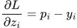 LaTeX:
\frac{\partial L}{\partial z_i}=p_i-y_iYaad rakhne ka cue: Softmax + CCE together: p minus y. Extra sigmoid slope nahi.
Solution — step by step
A logit is the raw score before softmax. Subtract each target entry from its matching probability entry.
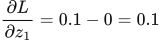 LaTeX:
\frac{\partial L}{\partial z_1}=0.1-0=0.1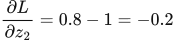 LaTeX:
\frac{\partial L}{\partial z_2}=0.8-1=-0.2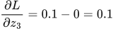 LaTeX:
\frac{\partial L}{\partial z_3}=0.1-0=0.1Final answer: [0.1, −0.2, 0.1]. Do not multiply these by a separate sigmoid derivative or by p(1−p). A mean over several examples introduces the corresponding averaging factor.
Sigmoid+BCE logit gradient: p=0.8, y=1
Question. A sigmoid output is p = 0.8 and target y = 1. For binary cross-entropy on one example, find the derivative with respect to the pre-sigmoid score z.
Given
p = 0.8; y = 1; single-example BCE; p = sigmoid(z).
To find
dL/dz, not dL/dp.
Formula — which one and why
Apply the chain rule to BCE followed backward through sigmoid. The factors p(1−p) cancel, leaving p−y.
p is an activated probability; z is its raw score; the requested derivative is with respect to z.
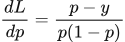 LaTeX:
\frac{dL}{dp}=\frac{p-y}{p(1-p)}LaTeX: \frac{dp}{dz}=p(1-p) LaTeX:
\frac{dL}{dz}=p-yYaad rakhne ka cue: BCE + sigmoid together ka shortcut p−y; chain already included.
Solution — step by step
Step 1: calculate the sigmoid slope.
 LaTeX:
p(1-p)=0.8(0.2)=0.16Step 2: differentiate BCE with respect to p.
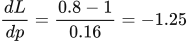 LaTeX:
\frac{dL}{dp}=\frac{0.8-1}{0.16}=-1.25Step 3: multiply the two local derivatives.
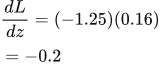 LaTeX:
\frac{dL}{dz}=(-1.25)(0.16)=-0.2Final answer: dL/dz = -0.2. No further sigmoid derivative is needed.
Sigmoid+BCE logit gradient: p=0.8, y=0
Question. A sigmoid output is p = 0.8 and target y = 0. For binary cross-entropy on one example, find the derivative with respect to the pre-sigmoid score z.
Given
p = 0.8; y = 0; single-example BCE; p = sigmoid(z).
To find
dL/dz, not dL/dp.
Formula — which one and why
Apply the chain rule to BCE followed backward through sigmoid. The factors p(1−p) cancel, leaving p−y.
p is an activated probability; z is its raw score; the requested derivative is with respect to z.
LaTeX: \frac{dL}{dp}=\frac{p-y}{p(1-p)}LaTeX: \frac{dp}{dz}=p(1-p)LaTeX: \frac{dL}{dz}=p-yYaad rakhne ka cue: BCE + sigmoid together ka shortcut p−y; chain already included.
Solution — step by step
Step 1: calculate the sigmoid slope.
LaTeX: p(1-p)=0.8(0.2)=0.16Step 2: differentiate BCE with respect to p.
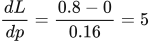 LaTeX:
\frac{dL}{dp}=\frac{0.8-0}{0.16}=5Step 3: multiply the two local derivatives.
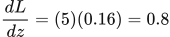 LaTeX:
\frac{dL}{dz}=(5)(0.16)=0.8Final answer: dL/dz = 0.8. No further sigmoid derivative is needed.
Hidden delta, weight gradient and bias gradient
A hidden neuron can influence several outputs. Add all those backward contributions before multiplying by its own activation derivative. For each connection, use the receiving neuron’s delta and the sending neuron’s activation. Keep the old weights unchanged until all gradients have been found.
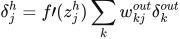 LaTeX:
\delta_j^h=f\prime(z_j^h)\sum_k w_{kj}^{out}\delta_k^{out}LaTeX: \frac{\partial L}{\partial w_{ji}}=\delta_j a_iLaTeX: \frac{\partial L}{\partial b_j}=\delta_jMore outputs and vectorized backpropagation
Definition. Vectorized backpropagation expresses the chain rule using matrix products and elementwise derivatives. When a hidden activation affects several outputs, its derivative contains the sum of the contributions from every downstream path.
Why the hidden derivative is a sum
If hidden activation hⱼ connects to output preactivations zₒ₁ and zₒ₂, changing hⱼ changes both outputs. The multivariable chain rule gives:
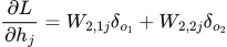 LaTeX:
\frac{\partial L}{\partial h_j}=W_{2,1j}\delta_{o_1}+W_{2,2j}\delta_{o_2}For any number of connected outputs, sum their contributions and then differentiate the hidden activation:
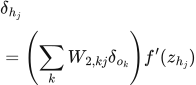 LaTeX:
\delta_{h_j}=\left(\sum_k W_{2,kj}\delta_{o_k}\right)f'(z_{h_j})Use the connecting weights from the original forward pass. Adding only the contribution of the first output would omit a dependency of the loss.
Matrix equations for one training sample
Use column vectors throughout. Let W₁ map d inputs to m hidden units and W₂ map those units to k outputs. The following output-delta formula assumes half sum of squared errors and an elementwise output activation f₂:
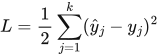 LaTeX:
L=\frac12\sum_{j=1}^{k}(\hat y_j-y_j)^2 LaTeX:
\delta_2=(\hat y-y)\odot f_2'(z_2)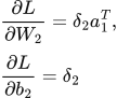 LaTeX:
\frac{\partial L}{\partial W_2}=\delta_2a_1^T,\qquad\frac{\partial L}{\partial b_2}=\delta_2 LaTeX:
\delta_1=(W_2^T\delta_2)\odot f_1'(z_1)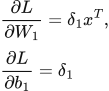 LaTeX:
\frac{\partial L}{\partial W_1}=\delta_1x^T,\qquad\frac{\partial L}{\partial b_1}=\delta_1Here ⊙ means elementwise multiplication. The product δ₂a₁ᵀ is an outer product: every receiving delta is multiplied by every sending activation.
| Quantity | Shape | Reason |
|---|---|---|
| W₁ and its gradient | m × d | m receiving hidden neurons, d inputs |
| W₂ and its gradient | k × m | k receiving output neurons, m hidden activations |
| δ₂ | k × 1 | One derivative per output preactivation |
| W₂ᵀδ₂ | m × 1 | The summed downstream derivative for each hidden unit |
| δ₂a₁ᵀ | (k × 1)(1 × m) = k × m | The output-weight gradient has the same shape as W₂ |
How the loss changes the output delta
For MSE averaged over k output components, the squared-error derivative has the factor 2/k. For sigmoid with binary cross-entropy, or softmax with categorical cross-entropy and a normalized target, the paired derivative simplifies to prediction minus target:
 LaTeX:
\delta_{\mathrm{output}}=\hat y-yThat simplification already includes differentiation of the paired activation and loss. Multiplying by a sigmoid derivative again would be incorrect. For sigmoid with half squared error, the sigmoid derivative is still required.
For a batch, sum per-example parameter gradients; divide by the batch size only if the objective is a batch mean. State the output reduction and batch reduction separately when both appear in a question.
Backpropagation with one hidden neuron
Definition. Backpropagation computes the derivatives of a scalar objective with respect to network parameters by applying the chain rule in reverse through the computational graph. An optimizer then uses these derivatives to update the parameters.
Network equations and the meaning of delta
Consider one input, one hidden neuron and one output neuron:
LaTeX: z_h=w_1x+b_1,\qquad h=f(z_h)LaTeX: z_o=w_2h+b_2,\qquad\hat y=g(z_o)For the half squared loss used in this example:
LaTeX: L=\frac12(\hat y-y)^2Define a neuron's delta as the derivative of the loss with respect to its preactivation, not with respect to its output:
LaTeX: \delta_o=\frac{\partial L}{\partial z_o}=(\hat y-y)g'(z_o)The output-weight derivative contains the hidden activation because zₒ = w₂h + b₂:
LaTeX: \frac{\partial L}{\partial w_2}=\delta_o h,\qquad\frac{\partial L}{\partial b_2}=\delta_oTo reach the hidden neuron, continue backwards through the old output weight and the hidden activation:
LaTeX: \delta_h=\delta_o w_2 f'(z_h)LaTeX: \frac{\partial L}{\partial w_1}=\delta_h x,\qquad\frac{\partial L}{\partial b_1}=\delta_hThe bias derivative equals the corresponding delta because the derivative of z with respect to its additive bias is 1. All these derivatives belong to the same forward pass; an updated weight must not be used partway through this backward pass.
Complete worked numerical
Question. x = 2, y = 1; w₁ = 0.5, b₁ = 0.1; w₂ = 0.8, b₂ = 0.2. Both neurons use ReLU. Use half squared loss. Find the output and all four parameter gradients, then update all four parameters using η = 0.1.
Given
x = 2, y = 1.
w₁ = 0.5, b₁ = 0.1.
w₂ = 0.8, b₂ = 0.2.
Both neurons use ReLU.
Use half squared loss.
Find the output and all four parameter gradients, then update all four parameters using η = 0.1.
To find
Find all preactivations, hidden activations and final outputs. Calculate the half summed squared loss and its output derivatives. Find the requested deltas and parameter gradients, then update the specified parameters.
Formula — which one and why
Forward propagation. Evaluate one layer completely before supplying its activated outputs to the next layer. Each layer has its own weights and biases.
x = input vector; h = hidden outputs; W₁,b₁ = hidden parameters; W₂,b₂ = output parameters; f₁,f₂ = the stated activations.
LaTeX: z_h=W_1x+b_1LaTeX: h=f_1(z_h)LaTeX: z_o=W_2h+b_2LaTeX: o=f_2(z_o)Yaad rakhne ka cue: Pehli layer ka activated output hi agli layer ka input hai.
Half summed squared loss. This loss convention takes one-half of the sum of squared prediction errors. Use it when the question specifies it, or explicitly state it as an assumption when the paper omits the loss. Differentiating cancels the factor one-half against the square derivative.
oⱼ = output j; yⱼ = target j; L = half summed squared loss under the stated or explicitly assumed convention.
LaTeX: L=\frac12\sum_j(o_j-y_j)^2LaTeX: \frac{\partial L}{\partial o_j}=o_j-y_jYaad rakhne ka cue: Half aur square ka 2 cancel: output derivative = prediction − target.
Backpropagation. The loss tells us how each output must change. Multiply by that neuron’s activation slope to obtain its delta. A weight gradient is receiving delta × sending value. Hidden deltas must include every outgoing path.
δ (delta) = derivative of loss with respect to a neuron’s preactivation; f′ = activation derivative; aᵢ = sending activation; Wⱼᵢ = connection weight. Use the exact loss scaling in the question.
LaTeX: \delta_{o_j}=\frac{\partial L}{\partial o_j}f_o\prime(z_{o_j})LaTeX: \delta_{h_i}=f_h\prime(z_{h_i})\sum_jW_{ji}^{(2)}\delta_{o_j}LaTeX: \frac{\partial L}{\partial W_{ji}}=\delta_ja_iLaTeX: \frac{\partial L}{\partial b_j}=\delta_jLaTeX: W_{ji,\mathrm{new}}=W_{ji}-\eta\frac{\partial L}{\partial W_{ji}}Yaad rakhne ka cue: Receiving delta × sending value = us connection ka gradient.
Solution — step by step
Step 1: forward propagation through the hidden neuron.
LaTeX: z_h=0.5(2)+0.1=1.1LaTeX: h=\operatorname{ReLU}(1.1)=1.1Step 2: forward propagation through the output neuron.
LaTeX: z_o=0.8(1.1)+0.2=1.08LaTeX: \hat y=\operatorname{ReLU}(1.08)=1.08ReLU is not bounded above by 1, so this output is valid. It is not being interpreted as a probability here.
Step 3: calculate the loss and output delta.
LaTeX: L=\frac12(1.08-1)^2=0.0032Both preactivations are positive, so both ReLU derivatives are 1.
LaTeX: \delta_o=(1.08-1)(1)=0.08Step 4: calculate the output-layer parameter gradients.
LaTeX: \frac{\partial L}{\partial w_2}=0.08(1.1)=0.088LaTeX: \frac{\partial L}{\partial b_2}=0.08Step 5: propagate the derivative to the hidden neuron.
Use w₂ = 0.8, its value during the forward pass:
LaTeX: \delta_h=0.08(0.8)(1)=0.064LaTeX: \frac{\partial L}{\partial w_1}=0.064(2)=0.128LaTeX: \frac{\partial L}{\partial b_1}=0.064Step 6: update each parameter using its own gradient.
LaTeX: w_{1,\mathrm{new}}=0.5-0.1(0.128)=0.4872LaTeX: b_{1,\mathrm{new}}=0.1-0.1(0.064)=0.0936LaTeX: w_{2,\mathrm{new}}=0.8-0.1(0.088)=0.7912LaTeX: b_{2,\mathrm{new}}=0.2-0.1(0.08)=0.192| Parameter | Gradient from the original forward pass | Updated value |
|---|---|---|
| w₁ | 0.128 | 0.4872 |
| b₁ | 0.064 | 0.0936 |
| w₂ | 0.088 | 0.7912 |
| b₂ | 0.08 | 0.192 |
Final answer: the original prediction is 1.08 and its loss is 0.0032. The table contains all requested gradients and updated parameters. A new forward pass would use all four new parameters together.
Drill 11 Full ReLU backpropagation
Question
Question. Input x = [1, 2]. Each row below lists the incoming weights of one receiving neuron. W₁ is shown below; b₁ = [0.1, 0.2]; W₂ is shown below; b₂ = [0.1]. Hidden and output activations are ReLU. Target y = [1]. Learning rate η = 0.1. Use half squared loss and update all weights and biases.
Answer — step by step
Given
Input x = [1, 2].
W₁ is printed with the question.
b₁ = [0.1, 0.2].
W₂ is printed with the question.
b₂ = [0.1].
Hidden and output activations are ReLU.
Target y = [1].
Learning rate η = 0.1.
Use half squared loss and update all weights and biases.
To find
Find all preactivations, hidden activations and final outputs. Calculate the half summed squared loss and its output derivatives. Find the requested deltas and parameter gradients, then update the specified parameters.
Formula — which one and why
Forward propagation. Evaluate one layer completely before supplying its activated outputs to the next layer. Each layer has its own weights and biases.
x = input vector; h = hidden outputs; W₁,b₁ = hidden parameters; W₂,b₂ = output parameters; f₁,f₂ = the stated activations.
LaTeX: z_h=W_1x+b_1LaTeX: h=f_1(z_h)LaTeX: z_o=W_2h+b_2LaTeX: o=f_2(z_o)Yaad rakhne ka cue: Pehli layer ka activated output hi agli layer ka input hai.
Half summed squared loss. This loss convention takes one-half of the sum of squared prediction errors. Use it when the question specifies it, or explicitly state it as an assumption when the paper omits the loss. Differentiating cancels the factor one-half against the square derivative.
oⱼ = output j; yⱼ = target j; L = half summed squared loss under the stated or explicitly assumed convention.
LaTeX: L=\frac12\sum_j(o_j-y_j)^2LaTeX: \frac{\partial L}{\partial o_j}=o_j-y_jYaad rakhne ka cue: Half aur square ka 2 cancel: output derivative = prediction − target.
Backpropagation. The loss tells us how each output must change. Multiply by that neuron’s activation slope to obtain its delta. A weight gradient is receiving delta × sending value. Hidden deltas must include every outgoing path.
δ (delta) = derivative of loss with respect to a neuron’s preactivation; f′ = activation derivative; aᵢ = sending activation; Wⱼᵢ = connection weight. Use the exact loss scaling in the question.
LaTeX: \delta_{o_j}=\frac{\partial L}{\partial o_j}f_o\prime(z_{o_j})LaTeX: \delta_{h_i}=f_h\prime(z_{h_i})\sum_jW_{ji}^{(2)}\delta_{o_j}LaTeX: \frac{\partial L}{\partial W_{ji}}=\delta_ja_iLaTeX: \frac{\partial L}{\partial b_j}=\delta_jLaTeX: W_{ji,\mathrm{new}}=W_{ji}-\eta\frac{\partial L}{\partial W_{ji}}Yaad rakhne ka cue: Receiving delta × sending value = us connection ka gradient.
Solution — step by step
Formulas used before substituting numbers
For every receiving neuron, z is its weighted sum and a is its activated output. The half squared loss sums the errors from all output neurons.
LaTeX: z_j=\sum_iw_{ji}a_i+b_j,\quad a_j=f(z_j),\quad L=\frac12\sum_k(o_k-y_k)^2Delta means the loss gradient with respect to a neuron's raw score. First calculate output deltas, then hidden deltas using every connected output path.
LaTeX: \delta_{o_k}=(o_k-y_k)f'(z_{o_k})LaTeX: \delta_{h_j}=\left(\sum_kw_{kj}\delta_{o_k}\right)f'(z_{h_j})The gradient of a connection is its receiving delta multiplied by its sending activation. A bias receives the constant 1.
LaTeX: \frac{\partial L}{\partial w_{ji}}=\delta_j a_i,\qquad \frac{\partial L}{\partial b_j}=\delta_jLaTeX: w_{ji,\mathrm{new}}=w_{ji}-\eta\delta_j a_i,\quad b_{j,\mathrm{new}}=b_j-\eta\delta_jFor sigmoid, use f′ = a(1 − a). For ReLU, use f′ = 1 for a positive raw score and 0 for a negative raw score. Store the old weights until all gradients have been calculated.
Step 1 map the arrows. Each row of W₁ receives all inputs; each row of W₂ receives all hidden outputs. Bias is added once per receiving neuron. All gradients below use the OLD weights from this same forward pass.
Hidden neuron 1:
LaTeX: z_{h_1} = (0.2 \times 1) + (0.1 \times 2) + (0.1) = 0.5LaTeX: h_{1} = \max(0,0.5) = 0.5Hidden neuron 2:
LaTeX: z_{h_2} = (0.3 \times 1) + (-0.1 \times 2) + (0.2) = 0.3LaTeX: h_{2} = \max(0,0.3) = 0.3Output neuron 1:
LaTeX: z_{o_1} = (0.4 \times 0.5) + (0.5 \times 0.3) + (0.1) = 0.45LaTeX: o_{1} = \max(0,0.45) = 0.45Step 2 loss convention. This worked solution uses half summed squared loss, L = ½Σ(o − y)². Follow the loss specified in the question; where none is supplied, this is an explicit assumption.
Prediction minus target = [-0.55]. Squared errors = [0.3025]. Half-sum squared loss = 0.15125; mean squared error = 0.3025. These are different unless the number of output components makes the scale coincide.
Output delta 1:
LaTeX: \delta_{o_1} = 1 \times (0.45-1) \times 1 = -0.55The ReLU derivative is 1 here because this preactivation is positive.
Step 3 output weights. Gradient = receiving delta × sending activation. An output bias gradient equals its delta.
h1 → o1:
Subtract η × gradient = −0.0275. This weight increases.
The sending value and receiving delta have different roles. All deltas still use the original forward-pass weights.
The receiving neuron supplies the delta; the sending neuron supplies its activation.
LaTeX: g_{1,1}^{(2)}=\frac{\partial L}{\partial W^{(2)}_{1,1}}=\delta_{o_1}h_1LaTeX: g_{1,1}^{(2)}=(-0.55)\times(0.5)\approx -0.275Apply the learning rate to this gradient and subtract the result from the old weight.
LaTeX: W^{(2)}_{1,1,\mathrm{new}}=0.4-0.1(-0.275)\approx 0.4275h2 → o1:
Subtract η × gradient = −0.0165. This weight increases.
The sending value and receiving delta have different roles. All deltas still use the original forward-pass weights.
The receiving neuron supplies the delta; the sending neuron supplies its activation.
LaTeX: g_{1,2}^{(2)}=\frac{\partial L}{\partial W^{(2)}_{1,2}}=\delta_{o_1}h_2LaTeX: g_{1,2}^{(2)}=(-0.55)\times(0.3)\approx -0.165Apply the learning rate to this gradient and subtract the result from the old weight.
LaTeX: W^{(2)}_{1,2,\mathrm{new}}=0.5-0.1(-0.165)\approx 0.5165Step 4 hidden deltas. A hidden unit can influence EVERY connected output, so add those paths BEFORE multiplying by the hidden activation derivative.
Hidden 1 downstream contribution:
Calculate each outgoing path using the old outgoing weight and that output's delta.
Multiply within each path. Add the resulting contributions at the shared hidden neuron.
Contribution from output 1.
LaTeX: C_1=(0.4)\times(-0.55)\approx -0.22Accumulate the contributions, then apply the hidden activation derivative below.
LaTeX: \text{Sum}=C_1\approx -0.22LaTeX: \delta_{h_1} = -0.22 \times 1 = -0.22Hidden 2 downstream contribution:
Calculate each outgoing path using the old outgoing weight and that output's delta.
Multiply within each path. Add the resulting contributions at the shared hidden neuron.
Contribution from output 1.
LaTeX: C_1=(0.5)\times(-0.55)\approx -0.275Accumulate the contributions, then apply the hidden activation derivative below.
LaTeX: \text{Sum}=C_1\approx -0.275LaTeX: \delta_{h_2} = -0.275 \times 1 = -0.275Step 5 input weights. Multiply the hidden delta by the corresponding raw input, not by the hidden output.
x1 → h1:
Subtract η × gradient = −0.022. This weight increases.
The sending value and receiving delta have different roles. All deltas still use the original forward-pass weights.
The receiving neuron supplies the delta; the sending neuron supplies the input value.
LaTeX: g_{1,1}^{(1)}=\frac{\partial L}{\partial W^{(1)}_{1,1}}=\delta_{h_1}x_1LaTeX: g_{1,1}^{(1)}=(-0.22)\times(1)\approx -0.22Apply the learning rate to this gradient and subtract the result from the old weight.
LaTeX: W^{(1)}_{1,1,\mathrm{new}}=0.2-0.1(-0.22)\approx 0.222x2 → h1:
Subtract η × gradient = −0.044. This weight increases.
The sending value and receiving delta have different roles. All deltas still use the original forward-pass weights.
The receiving neuron supplies the delta; the sending neuron supplies the input value.
LaTeX: g_{1,2}^{(1)}=\frac{\partial L}{\partial W^{(1)}_{1,2}}=\delta_{h_1}x_2LaTeX: g_{1,2}^{(1)}=(-0.22)\times(2)\approx -0.44Apply the learning rate to this gradient and subtract the result from the old weight.
LaTeX: W^{(1)}_{1,2,\mathrm{new}}=0.1-0.1(-0.44)\approx 0.144x1 → h2:
Subtract η × gradient = −0.0275. This weight increases.
The sending value and receiving delta have different roles. All deltas still use the original forward-pass weights.
The receiving neuron supplies the delta; the sending neuron supplies the input value.
LaTeX: g_{2,1}^{(1)}=\frac{\partial L}{\partial W^{(1)}_{2,1}}=\delta_{h_2}x_1LaTeX: g_{2,1}^{(1)}=(-0.275)\times(1)\approx -0.275Apply the learning rate to this gradient and subtract the result from the old weight.
LaTeX: W^{(1)}_{2,1,\mathrm{new}}=0.3-0.1(-0.275)\approx 0.3275x2 → h2:
Subtract η × gradient = −0.055. This weight increases.
The sending value and receiving delta have different roles. All deltas still use the original forward-pass weights.
The receiving neuron supplies the delta; the sending neuron supplies the input value.
LaTeX: g_{2,2}^{(1)}=\frac{\partial L}{\partial W^{(1)}_{2,2}}=\delta_{h_2}x_2LaTeX: g_{2,2}^{(1)}=(-0.275)\times(2)\approx -0.55Apply the learning rate to this gradient and subtract the result from the old weight.
LaTeX: W^{(1)}_{2,2,\mathrm{new}}=-0.1-0.1(-0.55)\approx -0.045Step 6 bias updates. A bias receives a constant input 1, so its gradient equals the corresponding delta. Use the same old forward pass and learning rate as the weight updates.
LaTeX: b_{h_1,\mathrm{new}}=0.1-0.1(-0.220000000)=0.122000000LaTeX: b_{h_2,\mathrm{new}}=0.2-0.1(-0.275000000)=0.227500000LaTeX: b_{o_1,\mathrm{new}}=0.1-0.1(-0.550000000)=0.155000000These are independent per-neuron biases. If the question fixes biases, keep them fixed. If it specifies a single tied bias, add all deltas sharing that bias before updating it.
Drill 12 Two output sigmoid backpropagation
Question
Question. Input x = [0.2, 0.4]. Each row below lists the incoming weights of one receiving neuron. W₁ is shown below; b₁ = [0.1, 0.1]; W₂ is shown below; b₂ = [0, 0.1]. Hidden and output activations are sigmoid. Target y = [1, 0]. Learning rate η = 0.2. Use half summed squared loss and update all parameters.
Answer — step by step
Given
Input x = [0.2, 0.4].
W₁ is printed with the question.
b₁ = [0.1, 0.1].
W₂ is printed with the question.
b₂ = [0, 0.1].
Hidden and output activations are sigmoid.
Target y = [1, 0].
Learning rate η = 0.2.
Use half summed squared loss and update all parameters.
To find
Find all preactivations, hidden activations and final outputs. Calculate the half summed squared loss and its output derivatives. Find the sigmoid output and, if requested, its derivative. Find the requested deltas and parameter gradients, then update the specified parameters.
Formula — which one and why
Forward propagation. Evaluate one layer completely before supplying its activated outputs to the next layer. Each layer has its own weights and biases.
x = input vector; h = hidden outputs; W₁,b₁ = hidden parameters; W₂,b₂ = output parameters; f₁,f₂ = the stated activations.
LaTeX: z_h=W_1x+b_1LaTeX: h=f_1(z_h)LaTeX: z_o=W_2h+b_2LaTeX: o=f_2(z_o)Yaad rakhne ka cue: Pehli layer ka activated output hi agli layer ka input hai.
Half summed squared loss. This loss convention takes one-half of the sum of squared prediction errors. Use it when the question specifies it, or explicitly state it as an assumption when the paper omits the loss. Differentiating cancels the factor one-half against the square derivative.
oⱼ = output j; yⱼ = target j; L = half summed squared loss under the stated or explicitly assumed convention.
LaTeX: L=\frac12\sum_j(o_j-y_j)^2LaTeX: \frac{\partial L}{\partial o_j}=o_j-y_jYaad rakhne ka cue: Half aur square ka 2 cancel: output derivative = prediction − target.
Sigmoid and its slope. Use sigmoid when the neuron is specified to squash its preactivation into (0,1). Once its output is known, its derivative needs only output × (1−output).
z = preactivation; p = sigmoid output; e is the exponential base, not a prediction error in this formula.
LaTeX: p=\frac{1}{1+e^{-z}}LaTeX: \frac{dp}{dz}=p(1-p)Yaad rakhne ka cue: Sigmoid output p; uska slope p × (1−p).
Backpropagation. The loss tells us how each output must change. Multiply by that neuron’s activation slope to obtain its delta. A weight gradient is receiving delta × sending value. Hidden deltas must include every outgoing path.
δ (delta) = derivative of loss with respect to a neuron’s preactivation; f′ = activation derivative; aᵢ = sending activation; Wⱼᵢ = connection weight. Use the exact loss scaling in the question.
LaTeX: \delta_{o_j}=\frac{\partial L}{\partial o_j}f_o\prime(z_{o_j})LaTeX: \delta_{h_i}=f_h\prime(z_{h_i})\sum_jW_{ji}^{(2)}\delta_{o_j}LaTeX: \frac{\partial L}{\partial W_{ji}}=\delta_ja_iLaTeX: \frac{\partial L}{\partial b_j}=\delta_jLaTeX: W_{ji,\mathrm{new}}=W_{ji}-\eta\frac{\partial L}{\partial W_{ji}}Yaad rakhne ka cue: Receiving delta × sending value = us connection ka gradient.
Solution — step by step
Formulas used before substituting numbers
For every receiving neuron, z is its weighted sum and a is its activated output. The half squared loss sums the errors from all output neurons.
LaTeX: z_j=\sum_iw_{ji}a_i+b_j,\quad a_j=f(z_j),\quad L=\frac12\sum_k(o_k-y_k)^2Delta means the loss gradient with respect to a neuron's raw score. First calculate output deltas, then hidden deltas using every connected output path.
LaTeX: \delta_{o_k}=(o_k-y_k)f'(z_{o_k})LaTeX: \delta_{h_j}=\left(\sum_kw_{kj}\delta_{o_k}\right)f'(z_{h_j})The gradient of a connection is its receiving delta multiplied by its sending activation. A bias receives the constant 1.
LaTeX: \frac{\partial L}{\partial w_{ji}}=\delta_j a_i,\qquad \frac{\partial L}{\partial b_j}=\delta_jLaTeX: w_{ji,\mathrm{new}}=w_{ji}-\eta\delta_j a_i,\quad b_{j,\mathrm{new}}=b_j-\eta\delta_jFor sigmoid, use f′ = a(1 − a). For ReLU, use f′ = 1 for a positive raw score and 0 for a negative raw score. Store the old weights until all gradients have been calculated.
Step 1 map the arrows. Each row of W₁ receives all inputs; each row of W₂ receives all hidden outputs. Bias is added once per receiving neuron. All gradients below use the OLD weights from this same forward pass.
Hidden neuron 1:
LaTeX: z_{h_1} = (0.1 \times 0.2) + (0.2 \times 0.4) + (0.1) = 0.2LaTeX: h_{1}=\frac{1}{1+e^{-(0.2)}}=0.549833997Hidden neuron 2:
LaTeX: z_{h_2} = (-0.2 \times 0.2) + (0.3 \times 0.4) + (0.1) = 0.18LaTeX: h_{2}=\frac{1}{1+e^{-(0.18)}}=0.544878892Output neuron 1:
LaTeX: z_{o_1} = (0.2 \times 0.549833997) + (-0.1 \times 0.544878892) + (0) = 0.05547891LaTeX: o_{1}=\frac{1}{1+e^{-(0.05547891)}}=0.513866171Output neuron 2:
LaTeX: z_{o_2} = (0.3 \times 0.549833997) + (0.4 \times 0.544878892) + (0.1) = 0.482901756LaTeX: o_{2}=\frac{1}{1+e^{-(0.482901756)}}=0.618432848Step 2 loss convention. This worked solution uses half summed squared loss, L = ½Σ(o − y)². Follow the loss specified in the question; where none is supplied, this is an explicit assumption.
Prediction minus target = [-0.486133829, 0.618432848]. Squared errors = [0.2363261, 0.382459187]. Half-sum squared loss = 0.309392643; mean squared error = 0.309392643. These are different unless the number of output components makes the scale coincide.
Output delta 1:
LaTeX: \delta_{o_1} = 1 \times (0.513866171-1) \times 0.249807729 = -0.121439988The derivative is o(1−o).
Output delta 2:
LaTeX: \delta_{o_2} = 1 \times (0.618432848-0) \times 0.235973661 = 0.145933863The derivative is o(1−o).
Step 3 output weights. Gradient = receiving delta × sending activation. An output bias gradient equals its delta.
h1 → o1:
Subtract η × gradient = −0.013354367. This weight increases.
The sending value and receiving delta have different roles. All deltas still use the original forward-pass weights.
The receiving neuron supplies the delta; the sending neuron supplies its activation.
LaTeX: g_{1,1}^{(2)}=\frac{\partial L}{\partial W^{(2)}_{1,1}}=\delta_{o_1}h_1LaTeX: g_{1,1}^{(2)}=(-0.121439988)\times(0.549833997)\approx -0.066771834Apply the learning rate to this gradient and subtract the result from the old weight.
LaTeX: W^{(2)}_{1,1,\mathrm{new}}=0.2-0.2(-0.066771834)\approx 0.213354367h2 → o1:
Subtract η × gradient = −0.013234017. This weight increases.
The sending value and receiving delta have different roles. All deltas still use the original forward-pass weights.
The receiving neuron supplies the delta; the sending neuron supplies its activation.
LaTeX: g_{1,2}^{(2)}=\frac{\partial L}{\partial W^{(2)}_{1,2}}=\delta_{o_1}h_2LaTeX: g_{1,2}^{(2)}=(-0.121439988)\times(0.544878892)\approx -0.066170086Apply the learning rate to this gradient and subtract the result from the old weight.
LaTeX: W^{(2)}_{1,2,\mathrm{new}}=-0.1-0.2(-0.066170086)\approx -0.086765983h1 → o2:
Subtract η × gradient = 0.01604788. This weight decreases.
The sending value and receiving delta have different roles. All deltas still use the original forward-pass weights.
The receiving neuron supplies the delta; the sending neuron supplies its activation.
LaTeX: g_{2,1}^{(2)}=\frac{\partial L}{\partial W^{(2)}_{2,1}}=\delta_{o_2}h_1LaTeX: g_{2,1}^{(2)}=(0.145933863)\times(0.549833997)\approx 0.080239399Apply the learning rate to this gradient and subtract the result from the old weight.
LaTeX: W^{(2)}_{2,1,\mathrm{new}}=0.3-0.2(0.080239399)\approx 0.28395212h2 → o2:
Subtract η × gradient = 0.015903256. This weight decreases.
The sending value and receiving delta have different roles. All deltas still use the original forward-pass weights.
The receiving neuron supplies the delta; the sending neuron supplies its activation.
LaTeX: g_{2,2}^{(2)}=\frac{\partial L}{\partial W^{(2)}_{2,2}}=\delta_{o_2}h_2LaTeX: g_{2,2}^{(2)}=(0.145933863)\times(0.544878892)\approx 0.079516282Apply the learning rate to this gradient and subtract the result from the old weight.
LaTeX: W^{(2)}_{2,2,\mathrm{new}}=0.4-0.2(0.079516282)\approx 0.384096744Step 4 hidden deltas. A hidden unit can influence EVERY connected output, so add those paths BEFORE multiplying by the hidden activation derivative.
Hidden 1 downstream contribution:
Calculate each outgoing path using the old outgoing weight and that output's delta.
Multiply within each path. Add the resulting contributions at the shared hidden neuron.
Contribution from output 1.
LaTeX: C_1=(0.2)\times(-0.121439988)\approx -0.024287998Contribution from output 2.
LaTeX: C_2=(0.3)\times(0.145933863)\approx 0.043780159Accumulate the contributions, then apply the hidden activation derivative below.
LaTeX: \text{Sum}=C_1+C_2\approx 0.019492161LaTeX: \delta_{h_1} = 0.019492161 \times 0.247516573 = 0.004824633Hidden 2 downstream contribution:
Calculate each outgoing path using the old outgoing weight and that output's delta.
Multiply within each path. Add the resulting contributions at the shared hidden neuron.
Contribution from output 1.
LaTeX: C_1=(-0.1)\times(-0.121439988)\approx 0.012143999Contribution from output 2.
LaTeX: C_2=(0.4)\times(0.145933863)\approx 0.058373545Accumulate the contributions, then apply the hidden activation derivative below.
LaTeX: \text{Sum}=C_1+C_2\approx 0.070517544LaTeX: \delta_{h_2} = 0.070517544 \times 0.247985885 = 0.017487356Step 5 input weights. Multiply the hidden delta by the corresponding raw input, not by the hidden output.
x1 → h1:
Subtract η × gradient = 0.000192985. This weight decreases.
The sending value and receiving delta have different roles. All deltas still use the original forward-pass weights.
The receiving neuron supplies the delta; the sending neuron supplies the input value.
LaTeX: g_{1,1}^{(1)}=\frac{\partial L}{\partial W^{(1)}_{1,1}}=\delta_{h_1}x_1LaTeX: g_{1,1}^{(1)}=(0.004824633)\times(0.2)\approx 0.000964927Apply the learning rate to this gradient and subtract the result from the old weight.
LaTeX: W^{(1)}_{1,1,\mathrm{new}}=0.1-0.2(0.000964927)\approx 0.099807015x2 → h1:
Subtract η × gradient = 0.000385971. This weight decreases.
The sending value and receiving delta have different roles. All deltas still use the original forward-pass weights.
The receiving neuron supplies the delta; the sending neuron supplies the input value.
LaTeX: g_{1,2}^{(1)}=\frac{\partial L}{\partial W^{(1)}_{1,2}}=\delta_{h_1}x_2LaTeX: g_{1,2}^{(1)}=(0.004824633)\times(0.4)\approx 0.001929853Apply the learning rate to this gradient and subtract the result from the old weight.
LaTeX: W^{(1)}_{1,2,\mathrm{new}}=0.2-0.2(0.001929853)\approx 0.199614029x1 → h2:
Subtract η × gradient = 0.000699494. This weight decreases.
The sending value and receiving delta have different roles. All deltas still use the original forward-pass weights.
The receiving neuron supplies the delta; the sending neuron supplies the input value.
LaTeX: g_{2,1}^{(1)}=\frac{\partial L}{\partial W^{(1)}_{2,1}}=\delta_{h_2}x_1LaTeX: g_{2,1}^{(1)}=(0.017487356)\times(0.2)\approx 0.003497471Apply the learning rate to this gradient and subtract the result from the old weight.
LaTeX: W^{(1)}_{2,1,\mathrm{new}}=-0.2-0.2(0.003497471)\approx -0.200699494x2 → h2:
Subtract η × gradient = 0.001398988. This weight decreases.
The sending value and receiving delta have different roles. All deltas still use the original forward-pass weights.
The receiving neuron supplies the delta; the sending neuron supplies the input value.
LaTeX: g_{2,2}^{(1)}=\frac{\partial L}{\partial W^{(1)}_{2,2}}=\delta_{h_2}x_2LaTeX: g_{2,2}^{(1)}=(0.017487356)\times(0.4)\approx 0.006994942Apply the learning rate to this gradient and subtract the result from the old weight.
LaTeX: W^{(1)}_{2,2,\mathrm{new}}=0.3-0.2(0.006994942)\approx 0.298601012Step 6 bias updates. A bias receives a constant input 1, so its gradient equals the corresponding delta. Use the same old forward pass and learning rate as the weight updates.
LaTeX: b_{h_1,\mathrm{new}}=0.1-0.2(0.004824633)=0.099035073LaTeX: b_{h_2,\mathrm{new}}=0.1-0.2(0.017487356)=0.096502529LaTeX: b_{o_1,\mathrm{new}}=0-0.2(-0.121439988)=0.024287998LaTeX: b_{o_2,\mathrm{new}}=0.1-0.2(0.145933863)=0.070813227These are independent per-neuron biases. If the question fixes biases, keep them fixed. If it specifies a single tied bias, add all deltas sharing that bias before updating it.
Drill 13 A negative ReLU blocks this path
Question
Question. x = 2, w1 = −0.4, b1 = 0.1, w2 = 0.5, b2 = 0.2; hidden ReLU, linear output, y = 1, half squared loss. Find dw 1 and dw 2.
Answer — step by step
Given
x = 2; w₁ = −0.4; b₁ = 0.1; w₂ = 0.5; b₂ = 0.2.
Hidden activation: ReLU; output activation: linear.
Target y = 1; loss: half squared error.
To find
Find the gradients of w₁ and w₂ and explain any zero gradients.
Formula — which one and why
Forward propagation. Evaluate one layer completely before supplying its activated outputs to the next layer. Each layer has its own weights and biases.
x = input vector; h = hidden outputs; W₁,b₁ = hidden parameters; W₂,b₂ = output parameters; f₁,f₂ = the stated activations.
LaTeX: z_h=W_1x+b_1LaTeX: h=f_1(z_h)LaTeX: z_o=W_2h+b_2LaTeX: o=f_2(z_o)Yaad rakhne ka cue: Pehli layer ka activated output hi agli layer ka input hai.
Half summed squared loss. This loss convention takes one-half of the sum of squared prediction errors. Use it when the question specifies it, or explicitly state it as an assumption when the paper omits the loss. Differentiating cancels the factor one-half against the square derivative.
oⱼ = output j; yⱼ = target j; L = half summed squared loss under the stated or explicitly assumed convention.
LaTeX: L=\frac12\sum_j(o_j-y_j)^2LaTeX: \frac{\partial L}{\partial o_j}=o_j-y_jYaad rakhne ka cue: Half aur square ka 2 cancel: output derivative = prediction − target.
Backpropagation. The loss tells us how each output must change. Multiply by that neuron’s activation slope to obtain its delta. A weight gradient is receiving delta × sending value. Hidden deltas must include every outgoing path.
δ (delta) = derivative of loss with respect to a neuron’s preactivation; f′ = activation derivative; aᵢ = sending activation; Wⱼᵢ = connection weight. Use the exact loss scaling in the question.
LaTeX: \delta_{o_j}=\frac{\partial L}{\partial o_j}f_o\prime(z_{o_j})LaTeX: \delta_{h_i}=f_h\prime(z_{h_i})\sum_jW_{ji}^{(2)}\delta_{o_j}LaTeX: \frac{\partial L}{\partial W_{ji}}=\delta_ja_iLaTeX: \frac{\partial L}{\partial b_j}=\delta_jLaTeX: W_{ji,\mathrm{new}}=W_{ji}-\eta\frac{\partial L}{\partial W_{ji}}Yaad rakhne ka cue: Receiving delta × sending value = us connection ka gradient.
Solution — step by step
Formulas used
The hidden neuron uses ReLU, but the output is linear. “Linear output” means its weighted sum is already its output.
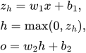 LaTeX:
z_h=w_1x+b_1,\quad h=\max(0,z_h),\quad o=w_2h+b_2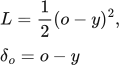 LaTeX:
L=\frac12(o-y)^2,\quad \delta_o=o-y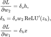 LaTeX:
\frac{\partial L}{\partial w_2}=\delta_o h,\quad \delta_h=\delta_o w_2\operatorname{ReLU}'(z_h),\quad \frac{\partial L}{\partial w_1}=\delta_h xStep 1: hidden weighted sum and activation
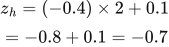 LaTeX:
z_h=(-0.4)\times2+0.1=-0.8+0.1=-0.7 LaTeX:
h=\max(0,-0.7)=0Because the raw hidden score is negative, ReLU's derivative at this point is 0.
Step 2: output prediction and output delta
 LaTeX:
o=0.5\times0+0.2=0.2 LaTeX:
\delta_o=0.2-1=-0.8Step 3: output weight gradient
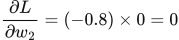 LaTeX:
\frac{\partial L}{\partial w_2}=(-0.8)\times0=0This is zero because the input to that connection, h, is zero.
Step 4: hidden delta and input weight gradient
 LaTeX:
\delta_h=(-0.8)\times0.5\times0=0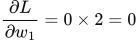 LaTeX:
\frac{\partial L}{\partial w_1}=0\times2=0Final answer: both requested weight gradients are zero. The output bias gradient equals −0.8, so a zero weight gradient does not mean every parameter's gradient is zero.
Gradient descent
A gradient tells us the local direction in which loss rises. Gradient descent subtracts a small multiple of that gradient. Learning rate η controls the size of this correction. After the first update, calculate the next gradient at the new parameter.
 LaTeX:
\theta_{new}=\theta-\eta g LaTeX:
g=\frac{\partial J}{\partial\theta}Reading an optimizer formula without getting lost
An optimizer updates the numbers the model is allowed to learn. Usually these are weights and biases. The letter θ is a convenient name for whichever parameter is currently being updated.
Old, current and new
At update t, θₜ₋₁ is the value before the update and θₜ is the value after it. The symbol gₜ is the loss gradient used in that update. If a question already supplies gₜ, use it. If it supplies a loss J(θ), differentiate J and evaluate the derivative at the stated position.
 LaTeX:
\theta_t=\theta_{t-1}-\eta g_tη, read eta, is the learning rate. It multiplies the gradient to determine the basic correction. A positive gradient is subtracted; a negative gradient makes the new value larger because subtracting a negative is addition.
What a stored state means
An optimizer may retain a number from its previous update. This number is called its state or memory. It is an ordinary calculated number, not an additional neuron. Momentum stores movement; AdaGrad stores a sum of squared gradients; RMSProp stores a moving average of squares; Adam stores a moving average of gradients and another of squares.
A weighted average from ordinary arithmetic
If the old state is 4, the new squared gradient is 9 and the decay is 0.9, retain 90% of the old state and add 10% of the new square.
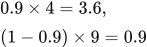 LaTeX:
0.9\times4=3.6,\qquad(1-0.9)\times9=0.9 LaTeX:
s_{\mathrm{new}}=3.6+0.9=4.5The coefficients 0.9 and 0.1 add to 1. As updates continue, a past contribution gets multiplied by 0.9 again, so its influence fades. AdaGrad instead gives 4 + 9 = 13 because it retains the full old sum.
Squared memory and signed direction
For gradient −3, the square is 9. The stored scale is positive, but the update still needs the negative gradient to determine direction. Do not replace every occurrence of g with g².
Epsilon and hats
ε, read epsilon, is a small positive number that prevents an exactly zero denominator. A hat in Adam, such as m with a hat, labels a bias-corrected average. A hat does not mean squaring. The power βᵗ uses the update number t, so its value changes from the first update to the second.
The ordinary gradient descent update
Definition. Gradient descent is an iterative first-order optimization algorithm that updates parameters in the negative direction of the current objective gradient, scaled by a positive learning rate.
Explanation and working
 LaTeX:
g_t=J\prime(\theta_{t-1})LaTeX: \theta_t=\theta_{t-1}-\eta g_tHere update numbers start at t = 1: calculate g₁ at θ₀, obtain θ₁, then calculate g₂ at θ₁. The subscript counts completed updates; it is not an exponent.
Read it aloud: “new parameter equals old parameter minus learning rate times current gradient.” The old parameter is where you are. The gradient gives the local uphill direction. The learning rate controls how far you move in the opposite direction.
Question. J(θ) = 0.7 θ³; θ₀ = 1; η = 0.1. Perform two iterations.
Given
J(θ) = 0.7θ³; initial θ₀ = 1; η = 0.1.
To find
Differentiate J and perform two gradient-descent iterations.
Formula — which one and why
Gradient descent. Evaluate the gradient at the current parameter, multiply by the learning rate and subtract. If the objective is supplied, differentiate it and recompute the gradient after each update.
θ (theta) = trainable parameter; g = derivative of the stated objective J; η = learning rate; t labels the update number.
LaTeX: g_t=J\prime(\theta_{t-1})LaTeX: \theta_t=\theta_{t-1}-\eta g_tYaad rakhne ka cue: Naya = purana − learning rate × current gradient.
Solution — step by step
Step 1. Differentiate. g(θ) = 0.7 × 3 × θ² = 2.1 θ².
Step 2. First update. g₁ = 2.1(1)² = 2.1. θ₁ = 1 − 0.1(2.1) = 0.79.
Step 3. Second gradient. Square the new value: 0.79² = 0.6241. Multiply: g₂ = 2.1 × 0.6241 = 1.31061.
Step 4. Second update. θ₂ = 0.79 − 0.1(1.31061) = 0.79 − 0.131061 = 0.658939.
The paper calls this SGD. With only a scalar objective supplied, no sample selection is specified; the arithmetic is the stated gradient-descent update. Also, this cubic is not bounded below over all real values. Do not claim these two steps prove convergence to a global minimum.
Common error: using the loss J itself instead of its derivative g. Another error is repeatedly using θ₀ to calculate later gradients.
Drill 16 GD variation 1
Question
Question. J(θ) = ½θ², θ₀ = 1, η = 0.1. Perform two GD updates.
Answer — step by step
Given
Objective: J(θ) = ½θ².
Initial θ₀ = 1; η = 0.1; two iterations.
To find
Find every stored state needed by the method and the parameter after each of two updates.
Formula — which one and why
Gradient descent. Evaluate the gradient at the current parameter, multiply by the learning rate and subtract. If the objective is supplied, differentiate it and recompute the gradient after each update.
θ (theta) = trainable parameter; g = derivative of the stated objective J; η = learning rate; t labels the update number.
LaTeX: g_t=J\prime(\theta_{t-1})LaTeX: \theta_t=\theta_{t-1}-\eta g_tYaad rakhne ka cue: Naya = purana − learning rate × current gradient.
Solution — step by step
Meaning of the symbols
θ (theta) is the number we update. η (eta) is learning rate 0.1. g is the derivative of the objective, evaluated at the required position. A subscript counts updates; θ₀ means the starting value.
Differentiate the objective first
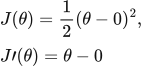 LaTeX:
J(\theta)=\frac12(\theta-0)^2,\qquad J\prime(\theta)=\theta-0The power rule brings down 2, which cancels the half. The inside derivative is 1, so the remaining gradient is θ minus 0.
Update formulas
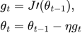 LaTeX:
g_t=J\prime(\theta_{t-1}),\quad \theta_t=\theta_{t-1}-\eta g_tStep 1: Update 1.
 LaTeX:
g_1=1-(0)=1 LaTeX:
\theta_1=1-0.1(1)=0.9Step 2: Update 2.
 LaTeX:
g_2=0.9-(0)=0.9 LaTeX:
\theta_2=0.9-0.1(0.9)=0.81Final parameter after two updates: 0.81. The second gradient is evaluated again using the parameter obtained after the first update.
Drill 17 GD variation 2
Question
Question. J(θ) = ½(θ−1)², θ₀ = -0.5, η = 0.1. Perform two GD updates.
Answer — step by step
Given
Objective: J(θ) = ½(θ−1)².
Initial θ₀ = −0.5; η = 0.1; two iterations.
To find
Find every stored state needed by the method and the parameter after each of two updates.
Formula — which one and why
Gradient descent. Evaluate the gradient at the current parameter, multiply by the learning rate and subtract. If the objective is supplied, differentiate it and recompute the gradient after each update.
θ (theta) = trainable parameter; g = derivative of the stated objective J; η = learning rate; t labels the update number.
LaTeX: g_t=J\prime(\theta_{t-1})LaTeX: \theta_t=\theta_{t-1}-\eta g_tYaad rakhne ka cue: Naya = purana − learning rate × current gradient.
Solution — step by step
Meaning of the symbols
θ (theta) is the number we update. η (eta) is learning rate 0.1. g is the derivative of the objective, evaluated at the required position. A subscript counts updates; θ₀ means the starting value.
Differentiate the objective first
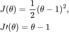 LaTeX:
J(\theta)=\frac12(\theta-1)^2,\qquad J\prime(\theta)=\theta-1The power rule brings down 2, which cancels the half. The inside derivative is 1, so the remaining gradient is θ minus 1.
Update formulas
LaTeX: g_t=J\prime(\theta_{t-1}),\quad \theta_t=\theta_{t-1}-\eta g_tStep 1: Update 1.
 LaTeX:
g_1=-0.5-(1)=-1.5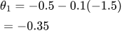 LaTeX:
\theta_1=-0.5-0.1(-1.5)=-0.35Step 2: Update 2.
 LaTeX:
g_2=-0.35-(1)=-1.35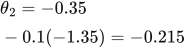 LaTeX:
\theta_2=-0.35-0.1(-1.35)=-0.215Final parameter after two updates: -0.215. The second gradient is evaluated again using the parameter obtained after the first update.
Drill 6 Chain rule on a tiny loss
Question
Question. Let o = wx+b, L = ½(o−y)², x = 3, w = 0.2, b = 0.1, y = 1. Find dL/dw, dL/db and update at η = 0.1.
Answer — step by step
Given
Model: o = wx+b; loss L = ½(o−y)².
x = 3; y = 1; w = 0.2; b = 0.1.
Learning rate η = 0.1.
To find
Find ∂L/∂w, ∂L/∂b and the updated weight and bias.
Formula — which one and why
Chain rule for a linear neuron. The weight changes the prediction, and the prediction changes the loss. Multiply those two local rates. Half squared loss differentiates to prediction minus target; the neuron contributes input x.
z = prediction; y = target; e = z−y; g_w and g_b = loss derivatives for weight and bias. ∂L/∂w means “how fast loss changes when w changes”. η (eta) = learning rate.
LaTeX: z=wx+bLaTeX: L=\frac12(z-y)^2LaTeX: g_w=\frac{\partial L}{\partial w}=(z-y)xLaTeX: g_b=\frac{\partial L}{\partial b}=z-yLaTeX: w_{\mathrm{new}}=w-\eta g_wLaTeX: b_{\mathrm{new}}=b-\eta g_bYaad rakhne ka cue: Ek path mein multiply; alag paths mil rahe hon toh add.
Solution — step by step
Meaning and formulas
The output o is a linear prediction: no sigmoid or ReLU is specified. Changing w changes o, which changes L. The chain rule multiplies those linked effects.
LaTeX: o=wx+b,\qquad L=\frac12(o-y)^2LaTeX: \frac{\partial L}{\partial o}=o-y,\quad \frac{\partial o}{\partial w}=x,\quad \frac{\partial o}{\partial b}=1LaTeX: \frac{\partial L}{\partial w}=(o-y)x,\qquad \frac{\partial L}{\partial b}=o-yThe learning rate η says how much of the gradient to subtract.
LaTeX: w_{\mathrm{new}}=w-\eta\frac{\partial L}{\partial w},\qquad b_{\mathrm{new}}=b-\eta\frac{\partial L}{\partial b}Step 1: obtain the current prediction and error
LaTeX: o=(0.2\times3)+0.1=0.6+0.1=0.7LaTeX: o-y=0.7-1=-0.3LaTeX: L=\frac12(-0.3)^2=\frac12(0.09)=0.045Step 2: calculate both gradients from this same prediction
LaTeX: \frac{\partial L}{\partial w}=(-0.3)\times3=-0.9LaTeX: \frac{\partial L}{\partial b}=(-0.3)\times1=-0.3Step 3: update the weight
LaTeX: w_{\mathrm{new}}=0.2-0.1(-0.9)=0.2-(-0.09)=0.29Step 4: update the bias
LaTeX: b_{\mathrm{new}}=0.1-0.1(-0.3)=0.1-(-0.03)=0.13Final answer: weight gradient −0.9; bias gradient −0.3; new weight 0.29; new bias 0.13. Both updates use the old forward pass.
Batch and mini-batch gradient
A batch is a group of training examples used together for one update. An epoch is one pass through the dataset. Averaging gradients and counting updates are different questions, so both receive complete worked examples below.
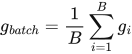 LaTeX:
g_{batch}=\frac1B\sum_{i=1}^{B}g_i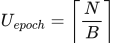 LaTeX:
U_{epoch}=\left\lceil\frac NB\right\rceilModel answer: batch, stochastic and mini-batch training
Question
Question. Differentiate batch gradient descent, stochastic gradient descent and mini-batch gradient descent. Explain an epoch, a batch and an iteration.
Answer — step by step
All three methods update model parameters using gradients. Their difference is the number of training examples used to estimate the gradient for one update.
A batch is the group of examples used together for an update. An iteration, in this context, is one optimizer update. An epoch is one complete pass through the chosen training dataset. One epoch usually contains several iterations.
| Basis | Batch GD | Stochastic GD | Mini-batch GD |
|---|---|---|---|
| Examples in one gradient | Entire training dataset | One example | A smaller group of B examples |
| Updates per epoch | One | N | Ceiling of N/B if the remainder is retained |
| Gradient behavior | Full-data gradient | Noisy sample gradient | Intermediate averaging |
| Practical implication | Updates can be expensive on large datasets | Many small, sequential updates | Common compromise for vectorized computation |
Example to distinguish the three counts
With 105 examples and batch size 20, five batches use 100 examples and a sixth uses the remaining 5. Therefore one epoch has 6 mini-batch updates. Three epochs give 18 updates. It would be 5 updates per epoch only if the problem explicitly discarded the incomplete batch.
The basic parameter update is unchanged:
 LaTeX:
\theta_{\mathrm{new}}=\theta_{\mathrm{old}}-\eta gFor batch or mini-batch training, g normally represents the gradient of the stated aggregate loss over that group. For sequential SGD, update after each example and use the new parameter for the next example. Consequently, one SGD epoch need not equal one batch update even when both use the same examples.
A tiny dataset shows why the methods differ
Question. Train ŷ = wx on samples (1,2) and (2,4), starting at w = 1, with η = 0.1 and mean half squared loss. Compare one batch update with one SGD epoch in the listed order.
Given
Model ŷ = wx; initial w = 1; η = 0.1.
Samples in order: (1,2), (2,4).
Mean half squared loss for the batch.
To find
Compare one batch update with a sequential SGD epoch.
Formula — which one and why
Batch mean versus sequential SGD. A batch update averages gradients evaluated at the same old parameter. Sequential SGD updates after each sample, so later samples use the changed parameter.
B = number of examples in the batch; gᵢ = sample gradient; η = learning rate. For the linear half squared objective, sample gradient is (wx−y)x.
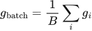 LaTeX:
g_{\mathrm{batch}}=\frac1B\sum_i g_i LaTeX:
g_i=(wx_i-y_i)x_i LaTeX:
w_{\mathrm{new}}=w-\eta gYaad rakhne ka cue: Batch: same old weight par average; SGD: har sample ke baad weight change.
Solution — step by step
One batch update
Step 1: predict sample 1 with the original weight.
 LaTeX:
\hat y_1=1(1)=1Step 2: calculate its error.
 LaTeX:
e_1=1-2=-1Step 3: multiply its error by its input.
 LaTeX:
g_1=(-1)(1)=-1Step 4: predict sample 2 with the same original weight.
 LaTeX:
\hat y_2=1(2)=2Step 5: calculate its error.
 LaTeX:
e_2=2-4=-2Step 6: multiply its error by its input.
 LaTeX:
g_2=(-2)(2)=-4Step 7: average the two gradients.
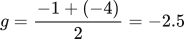 LaTeX:
g=\frac{-1+(-4)}2=-2.5Step 8: update once.
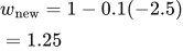 LaTeX:
w_{\mathrm{new}}=1-0.1(-2.5)=1.25One sequential SGD epoch
Step 1: use the first sample gradient.
 LaTeX:
g_1=-1Step 2: update after the first sample.
 LaTeX:
w_1=1-0.1(-1)=1.1Step 3: predict sample 2 using the changed weight.
 LaTeX:
\hat y_2=1.1(2)=2.2Step 4: find sample 2 error.
 LaTeX:
e_2=2.2-4=-1.8Step 5: find the new sample 2 gradient.
 LaTeX:
g_2=(-1.8)(2)=-3.6Step 6: update after sample 2.
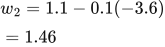 LaTeX:
w_2=1.1-0.1(-3.6)=1.46Final answer: batch weight = 1.25; sequential SGD weight = 1.46. SGD changes the weight between samples.
Larger mini-batches use more memory and often make better use of parallel hardware. Smaller batches provide noisier gradient estimates and more updates per epoch. Wall-clock speed and generalization depend on the implementation and problem, so “SGD always converges fastest” is not a safe claim.
Drill 14 Batch and sequential SGD
Question
Question. ŷ = wx, start w = 0, η = 0.1, data(1,1), (2,2). Use mean half squared loss for a batch. Compare one batch update with one sequential SGD epoch.
Answer — step by step
Given
Model ŷ = wx; initial w = 0; η = 0.1.
Samples in order: (x,y) = (1,1), then (2,2).
Batch objective: mean half squared loss.
To find
Compare the weight after one batch update and one sequential SGD epoch.
Formula — which one and why
Batch mean versus sequential SGD. A batch update averages gradients evaluated at the same old parameter. Sequential SGD updates after each sample, so later samples use the changed parameter.
B = number of examples in the batch; gᵢ = sample gradient; η = learning rate. For the linear half squared objective, sample gradient is (wx−y)x.
LaTeX: g_{\mathrm{batch}}=\frac1B\sum_i g_iLaTeX: g_i=(wx_i-y_i)x_iLaTeX: w_{\mathrm{new}}=w-\eta gYaad rakhne ka cue: Batch: same old weight par average; SGD: har sample ke baad weight change.
Solution — step by step
Meaning and formulas
For one sample, x is the input, y is the target, and w is the weight. Batch GD averages gradients evaluated at the same old weight. Sequential SGD updates after each sample and uses that new weight for the next sample.
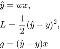 LaTeX:
\hat y=wx,\quad L=\frac12(\hat y-y)^2,\quad g=(\hat y-y)x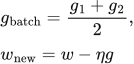 LaTeX:
g_{\mathrm{batch}}=\frac{g_1+g_2}{2},\qquad w_{\mathrm{new}}=w-\eta gStep 1: Part A: one batch update from w = 0.
For sample (1,1), prediction = 0 × 1 = 0, so:
 LaTeX:
g_1=(0-1)\times1=-1For sample (2,2), keep the same weight 0. Prediction = 0 × 2 = 0, so:
 LaTeX:
g_2=(0-2)\times2=-4Average these two gradients, then update once.
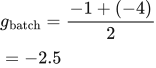 LaTeX:
g_{\mathrm{batch}}=\frac{-1+(-4)}2=-2.5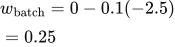 LaTeX:
w_{\mathrm{batch}}=0-0.1(-2.5)=0.25Step 2: Part B: one SGD epoch, restarting at w = 0.
The first sample has gradient −1, just as above.
 LaTeX:
w_1=0-0.1(-1)=0.1For the second sample use this new weight, so prediction is:
 LaTeX:
\hat y_2=0.1\times2=0.2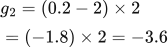 LaTeX:
g_2=(0.2-2)\times2=(-1.8)\times2=-3.6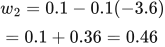 LaTeX:
w_2=0.1-0.1(-3.6)=0.1+0.36=0.46Final answer: batch result 0.25; sequential SGD result 0.46. The difference comes from the timing of the updates.
Drill 15 Incomplete mini batch
Question
Question. N = 103, B = 20, epochs = 3. Count updates for batch GD, SGD, mini-batch keeping the remainder, and mini-batch dropping it.
Answer — step by step
Given
N = 103 samples; B = 20 samples per mini-batch.
E = 3 epochs.
Compare both remainder policies: keep or drop the final 3 examples.
To find
Find total updates for full-batch GD, SGD, and both mini-batch policies.
Formula — which one and why
Number of updates. An update occurs after one processed batch. Full-batch GD uses one batch per epoch; SGD uses one sample per batch. Mini-batches need a stated remainder policy.
N = dataset size; B = batch size; E = number of epochs. Ceiling rounds upward to include a smaller final batch; floor drops it.
 LaTeX:
U_{\mathrm{batch}}=E LaTeX:
U_{\mathrm{SGD}}=EN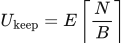 LaTeX:
U_{\mathrm{keep}}=E\left\lceil\frac NB\right\rceil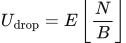 LaTeX:
U_{\mathrm{drop}}=E\left\lfloor\frac NB\right\rfloorYaad rakhne ka cue: Kitne batches process hue, utne updates hue.
Solution — step by step
Meaning and formulas
An epoch means one pass through the dataset. An update happens once per batch used. N is the number of samples, B is the chosen batch size, and E is the number of epochs.
 LaTeX:
U_{\mathrm{batch}}=E,\qquad U_{\mathrm{SGD}}=NE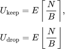 LaTeX:
U_{\mathrm{keep}}=E\left\lceil\frac NB\right\rceil,\qquad U_{\mathrm{drop}}=E\left\lfloor\frac NB\right\rfloorCeiling rounds up to the next integer; floor rounds down. The final incomplete batch needs an update only if it is retained.
Step 1: batch GD
All 103 samples form one batch per epoch.
 LaTeX:
U_{\mathrm{batch}}=3\times1=3Step 2: SGD
Each sample gets its own update.
 LaTeX:
U_{\mathrm{SGD}}=103\times3=309Step 3: mini-batches with the remainder
 LaTeX:
103=5\times20+3The batch sizes are 20, 20, 20, 20, 20 and 3. Six batches per epoch give:
 LaTeX:
U_{\mathrm{keep}}=6\times3=18Step 4: mini-batches without the remainder
Only the five complete batches are used each epoch.
 LaTeX:
U_{\mathrm{drop}}=5\times3=15Final answer: 3, 309, 18 and 15 updates respectively.
Momentum: signed velocity
Momentum carries some of the previous movement into the next update. Here v is signed movement, so the new parameter is the old parameter plus v. A negative v moves the parameter down. Use the same convention throughout the calculation.
 LaTeX:
v_t=\beta v_{t-1}-\eta g_t LaTeX:
\theta_t=\theta_{t-1}+v_tModel answer: momentum and Nesterov
Question
Question. Explain momentum and Nesterov accelerated gradient. How does the point at which the gradient is measured differ?
Answer — step by step
Momentum retains a fraction of the previous movement and combines it with the current gradient correction. Movement in a persistent direction can build up, while alternating directions can partially cancel. This can reduce zig-zagging and improve progress through poorly scaled regions.
Momentum formulas
This answer uses signed displacement velocity v: a negative velocity moves the parameter left. η is learning rate and β is the fraction of previous velocity retained.
 LaTeX:
g_t=J'(\theta_{t-1})LaTeX: v_t=\beta v_{t-1}-\eta g_tLaTeX: \theta_t=\theta_{t-1}+v_tNesterov's change
Nesterov first forms a lookahead position using the old momentum. It measures the gradient there, then computes a new velocity and updates the actual old parameter.
 LaTeX:
\theta_{\mathrm{look}}=\theta_{t-1}+\beta v_{t-1} LaTeX:
g_t=J'(\theta_{\mathrm{look}})The velocity and parameter update formulas remain as displayed above. Add the new velocity to θ at the previous iteration, not to the lookahead point.
| Basis | Momentum | Nesterov |
|---|---|---|
| Gradient evaluated at | Current parameter | Lookahead parameter |
| Information retained | Previous velocity | Previous velocity |
| Intuition | Continue useful movement | Inspect the slope where old momentum points |
| Initial zero velocity | No movement contribution yet | First lookahead equals current parameter |
Both require suitable learning rate and momentum settings. Neither guarantees the global minimum of a general neural-network objective. Different books use different definitions of stored velocity, so the definition and update must be used together consistently.
Momentum remembers movement
Definition. Momentum is a gradient-based optimization method that combines the current gradient correction with a fraction of the previous parameter displacement. It can accumulate movement along persistent directions and damp some oscillations across alternating directions.
Update equations and convention
This course uses signed displacement velocity v. It already includes the learning rate, and the parameter update adds it to the old parameter:
LaTeX: g_t=J'(\theta_{t-1})LaTeX: v_t=\beta v_{t-1}-\eta g_tLaTeX: \theta_t=\theta_{t-1}+v_tθ is the parameter, η is the learning rate and β controls how much previous displacement is retained, normally with 0 ≤ β < 1. A negative v moves θ in the negative direction. Every parameter has its own velocity; this optimizer state is distinct from the network's trainable parameters.
Complete numerical: two iterations
Question. J(θ) = ½θ², θ₀ = 1, v₀ = 0, η = 0.1, β = 0.9. Find two iterations using signed displacement velocity.
Given
J(θ) = ½θ²; θ₀ = 1; v₀ = 0.
η = 0.1; β = 0.9; signed-displacement velocity.
To find
Find the gradient, velocity and actual parameter after each of two iterations.
Formula — which one and why
Momentum with signed velocity. Combine the retained old displacement with the current downhill correction, then add that signed displacement to the old parameter.
v = signed velocity/displacement; β = momentum coefficient; g = current gradient; η = learning rate. This convention uses +v in the parameter update.
LaTeX: v_t=\beta v_{t-1}-\eta g_tLaTeX: \theta_t=\theta_{t-1}+v_tYaad rakhne ka cue: Pehle velocity banao; phir old parameter mein velocity jodo.
Solution — step by step
Derivative used: differentiating J gives J′(θ) = θ. The gradient must therefore be reevaluated at the current θ on each iteration.
Step 1: Iteration 1: gradient, velocity, parameter.
 LaTeX:
g_1=J'(1)=1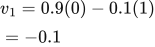 LaTeX:
v_1=0.9(0)-0.1(1)=-0.1 LaTeX:
\theta_1=1+(-0.1)=0.9Step 2: Iteration 2: use θ₁ and v₁.
 LaTeX:
g_2=J'(0.9)=0.9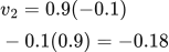 LaTeX:
v_2=0.9(-0.1)-0.1(0.9)=-0.18 LaTeX:
\theta_2=0.9+(-0.18)=0.72| Iteration | Parameter where gradient is evaluated | Gradient | New velocity | New parameter |
|---|---|---|---|---|
| 1 | 1 | 1 | −0.1 | 0.9 |
| 2 | 0.9 | 0.9 | −0.18 | 0.72 |
Final answer: θ₁ = 0.9 and θ₂ = 0.72. At iteration 2, the retained displacement contributes −0.09 and the new gradient correction contributes another −0.09. Their sum explains the larger displacement despite the smaller current gradient.
Properties and alternative notation
Momentum can improve progress through long, poorly scaled valleys, but excessive learning rate or momentum can overshoot. It does not guarantee a global minimum for a general neural-network objective.
Some texts store a positive gradient accumulator u instead:
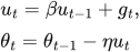 LaTeX:
u_t=\beta u_{t-1}+g_t,\qquad\theta_t=\theta_{t-1}-\eta u_tWith constant η and consistent initialization, this corresponds to vₜ = −ηuₜ. A normalized moving average containing (1−β)gₜ is a different scaling convention. Use the exact recurrence stated in the question instead of combining pieces of different conventions.
Drill 18 Momentum variation 1
Question
Question. J(θ) = ½θ², θ₀ = 1, η = 0.1. Perform two Momentum updates. Use β = 0.9, v₀ = 0 and signed velocity.
Answer — step by step
Given
Objective: J(θ) = ½θ².
Initial θ₀ = 1; η = 0.1; two iterations.
β = 0.9; initial signed velocity v₀ = 0.
To find
Find every stored state needed by the method and the parameter after each of two updates.
Formula — which one and why
Momentum with signed velocity. Combine the retained old displacement with the current downhill correction, then add that signed displacement to the old parameter.
v = signed velocity/displacement; β = momentum coefficient; g = current gradient; η = learning rate. This convention uses +v in the parameter update.
LaTeX: v_t=\beta v_{t-1}-\eta g_tLaTeX: \theta_t=\theta_{t-1}+v_tYaad rakhne ka cue: Pehle velocity banao; phir old parameter mein velocity jodo.
Solution — step by step
Meaning of the symbols
θ (theta) is the number we update. η (eta) is learning rate 0.1. g is the derivative of the objective, evaluated at the required position. A subscript counts updates; θ₀ means the starting value.
Differentiate the objective first
LaTeX: J(\theta)=\frac12(\theta-0)^2,\qquad J\prime(\theta)=\theta-0The power rule brings down 2, which cancels the half. The inside derivative is 1, so the remaining gradient is θ minus 0.
Update formulas
v stores the signed movement from the previous update. β = 0.9 retains 90% of that movement. Start v₀ = 0.
LaTeX: g_t=J\prime(\theta_{t-1})LaTeX: v_t=\beta v_{t-1}-\eta g_t,\quad \theta_t=\theta_{t-1}+v_tStep 1: Update 1.
LaTeX: g_1=1-(0)=1LaTeX: v_1=0.9(0)-0.1(1)=-0.1LaTeX: \theta_1=1+(-0.1)=0.9Step 2: Update 2.
LaTeX: g_2=0.9-(0)=0.9LaTeX: v_2=0.9(-0.1)-0.1(0.9)=-0.18LaTeX: \theta_2=0.9+(-0.18)=0.72Final parameter after two updates: 0.72. The second gradient is evaluated again using the parameter obtained after the first update.
Drill 19 Momentum variation 2
Question
Question. J(θ) = ½(θ−1)², θ₀ = -0.5, η = 0.1. Perform two Momentum updates. Use β = 0.9, v₀ = 0 and signed velocity.
Answer — step by step
Given
Objective: J(θ) = ½(θ−1)².
Initial θ₀ = −0.5; η = 0.1; two iterations.
β = 0.9; initial signed velocity v₀ = 0.
To find
Find every stored state needed by the method and the parameter after each of two updates.
Formula — which one and why
Momentum with signed velocity. Combine the retained old displacement with the current downhill correction, then add that signed displacement to the old parameter.
v = signed velocity/displacement; β = momentum coefficient; g = current gradient; η = learning rate. This convention uses +v in the parameter update.
LaTeX: v_t=\beta v_{t-1}-\eta g_tLaTeX: \theta_t=\theta_{t-1}+v_tYaad rakhne ka cue: Pehle velocity banao; phir old parameter mein velocity jodo.
Solution — step by step
Meaning of the symbols
θ (theta) is the number we update. η (eta) is learning rate 0.1. g is the derivative of the objective, evaluated at the required position. A subscript counts updates; θ₀ means the starting value.
Differentiate the objective first
LaTeX: J(\theta)=\frac12(\theta-1)^2,\qquad J\prime(\theta)=\theta-1The power rule brings down 2, which cancels the half. The inside derivative is 1, so the remaining gradient is θ minus 1.
Update formulas
v stores the signed movement from the previous update. β = 0.9 retains 90% of that movement. Start v₀ = 0.
LaTeX: g_t=J\prime(\theta_{t-1})LaTeX: v_t=\beta v_{t-1}-\eta g_t,\quad \theta_t=\theta_{t-1}+v_tStep 1: Update 1.
LaTeX: g_1=-0.5-(1)=-1.5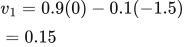 LaTeX:
v_1=0.9(0)-0.1(-1.5)=0.15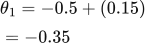 LaTeX:
\theta_1=-0.5+(0.15)=-0.35Step 2: Update 2.
LaTeX: g_2=-0.35-(1)=-1.35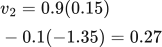 LaTeX:
v_2=0.9(0.15)-0.1(-1.35)=0.27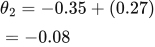 LaTeX:
\theta_2=-0.35+(0.27)=-0.08Final parameter after two updates: -0.08. The second gradient is evaluated again using the parameter obtained after the first update.
Nesterov: look-ahead gradient
Nesterov first uses the old movement to choose a temporary look-ahead position. It measures the gradient there, calculates the new movement, then adds that movement to the original parameter. The temporary look-ahead position does not replace the original parameter in the final addition.
 LaTeX:
\theta_{look}=\theta+\beta v LaTeX:
v_{new}=\beta v-\eta g(\theta_{look}) LaTeX:
\theta_{new}=\theta+v_{new}Nesterov looks before correcting
Definition. Nesterov accelerated gradient is a momentum-based method that evaluates the gradient at a lookahead parameter, formed using the previous velocity, before calculating the new velocity and actual parameter update.
What changes relative to momentum
Ordinary momentum evaluates J′ at θₜ₋₁. Nesterov evaluates it after the anticipated displacement βvₜ₋₁. This changes the point where the objective's slope is measured:
 LaTeX:
\theta_{\mathrm{look},t}=\theta_{t-1}+\beta v_{t-1} LaTeX:
g_t=J'(\theta_{\mathrm{look},t})LaTeX: v_t=\beta v_{t-1}-\eta g_tLaTeX: \theta_t=\theta_{t-1}+v_tThe lookahead point is an auxiliary evaluation point, not the new actual parameter. In this signed-displacement convention, the new velocity is added to θₜ₋₁.
Complete numerical: two iterations
Question. J(θ) = ½θ², θ₀ = 1, v₀ = 0, η = 0.1 and β = 0.9. Perform two Nesterov updates using signed displacement velocity.
Given
J(θ) = ½θ²; θ₀ = 1; v₀ = 0.
η = 0.1; β = 0.9; signed-displacement velocity.
To find
Find the gradient, velocity and actual parameter after each of two iterations.
Formula — which one and why
Nesterov lookahead. First look ahead using the old velocity. Measure the gradient there, form the new velocity, then add that velocity to the original current parameter.
θ_look = temporary gradient-evaluation point; v = signed displacement; β = momentum coefficient; η = learning rate.
LaTeX: \theta_{\mathrm{look}}=\theta_{t-1}+\beta v_{t-1} LaTeX:
g_t=J\prime(\theta_{\mathrm{look}})LaTeX: v_t=\beta v_{t-1}-\eta g_tLaTeX: \theta_t=\theta_{t-1}+v_tYaad rakhne ka cue: Pehle look ahead; gradient wahan; update original position se.
Solution — step by step
The derivative is J′(θ) = θ. Therefore the gradient equals the lookahead value in this particular objective.
Iteration 1 — step 1: locate the lookahead point.
 LaTeX:
\theta_{\mathrm{look},1}=1+0.9(0)=1Step 2: evaluate the gradient there.
LaTeX: g_1=J'(1)=1Step 3: calculate the new velocity and actual parameter.
LaTeX: v_1=0.9(0)-0.1(1)=-0.1LaTeX: \theta_1=1+(-0.1)=0.9Iteration 2 — step 1: use the previous actual parameter and velocity.
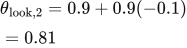 LaTeX:
\theta_{\mathrm{look},2}=0.9+0.9(-0.1)=0.81Step 2: evaluate the gradient at 0.81, not at 0.9.
 LaTeX:
g_2=J'(0.81)=0.81Step 3: calculate the new velocity.
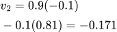 LaTeX:
v_2=0.9(-0.1)-0.1(0.81)=-0.171Step 4: update the old actual parameter.
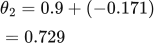 LaTeX:
\theta_2=0.9+(-0.171)=0.729| Iteration | Old actual θ | Lookahead θ | Gradient | New v | New actual θ |
|---|---|---|---|---|---|
| 1 | 1 | 1 | 1 | −0.1 | 0.9 |
| 2 | 0.9 | 0.81 | 0.81 | −0.171 | 0.729 |
Final answer: θ₁ = 0.9 and θ₂ = 0.729. The first update matches ordinary momentum because v₀ = 0. At the second update, ordinary momentum would use gradient 0.9 and produce θ₂ = 0.72. Adding v₂ to 0.81 instead of 0.9 would count the old momentum contribution twice.
Drill 20 Nesterov variation 1
Question
Question. J(θ) = ½θ², θ₀ = 1, η = 0.1. Perform two Nesterov updates. Use β = 0.9, v₀ = 0 and signed velocity.
Answer — step by step
Given
Objective: J(θ) = ½θ².
Initial θ₀ = 1; η = 0.1; two iterations.
β = 0.9; initial signed velocity v₀ = 0.
To find
Find every stored state needed by the method and the parameter after each of two updates.
Formula — which one and why
Nesterov lookahead. First look ahead using the old velocity. Measure the gradient there, form the new velocity, then add that velocity to the original current parameter.
θ_look = temporary gradient-evaluation point; v = signed displacement; β = momentum coefficient; η = learning rate.
LaTeX: \theta_{\mathrm{look}}=\theta_{t-1}+\beta v_{t-1}LaTeX: g_t=J\prime(\theta_{\mathrm{look}})LaTeX: v_t=\beta v_{t-1}-\eta g_tLaTeX: \theta_t=\theta_{t-1}+v_tYaad rakhne ka cue: Pehle look ahead; gradient wahan; update original position se.
Solution — step by step
Meaning of the symbols
θ (theta) is the number we update. η (eta) is learning rate 0.1. g is the derivative of the objective, evaluated at the required position. A subscript counts updates; θ₀ means the starting value.
Differentiate the objective first
LaTeX: J(\theta)=\frac12(\theta-0)^2,\qquad J\prime(\theta)=\theta-0The power rule brings down 2, which cancels the half. The inside derivative is 1, so the remaining gradient is θ minus 0.
Update formulas
v stores the signed movement from the previous update. β = 0.9 retains 90% of that movement. Start v₀ = 0.
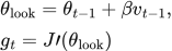 LaTeX:
\theta_{\mathrm{look}}=\theta_{t-1}+\beta v_{t-1},\quad g_t=J\prime(\theta_{\mathrm{look}})LaTeX: v_t=\beta v_{t-1}-\eta g_t,\quad \theta_t=\theta_{t-1}+v_tStep 1: Update 1.
 LaTeX:
\theta_{\mathrm{look}}=1+0.9(0)=1LaTeX: g_1=1-(0)=1LaTeX: v_1=0.9(0)-0.1(1)=-0.1LaTeX: \theta_1=1+(-0.1)=0.9Step 2: Update 2.
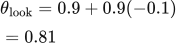 LaTeX:
\theta_{\mathrm{look}}=0.9+0.9(-0.1)=0.81 LaTeX:
g_2=0.81-(0)=0.81LaTeX: v_2=0.9(-0.1)-0.1(0.81)=-0.171LaTeX: \theta_2=0.9+(-0.171)=0.729Final parameter after two updates: 0.729. The lookahead locates the gradient; the new velocity is added to the old actual parameter, not to the lookahead.
Drill 21 Nesterov variation 2
Question
Question. J(θ) = ½(θ−1)², θ₀ = -0.5, η = 0.1. Perform two Nesterov updates. Use β = 0.9, v₀ = 0 and signed velocity.
Answer — step by step
Given
Objective: J(θ) = ½(θ−1)².
Initial θ₀ = −0.5; η = 0.1; two iterations.
β = 0.9; initial signed velocity v₀ = 0.
To find
Find every stored state needed by the method and the parameter after each of two updates.
Formula — which one and why
Nesterov lookahead. First look ahead using the old velocity. Measure the gradient there, form the new velocity, then add that velocity to the original current parameter.
θ_look = temporary gradient-evaluation point; v = signed displacement; β = momentum coefficient; η = learning rate.
LaTeX: \theta_{\mathrm{look}}=\theta_{t-1}+\beta v_{t-1}LaTeX: g_t=J\prime(\theta_{\mathrm{look}})LaTeX: v_t=\beta v_{t-1}-\eta g_tLaTeX: \theta_t=\theta_{t-1}+v_tYaad rakhne ka cue: Pehle look ahead; gradient wahan; update original position se.
Solution — step by step
Meaning of the symbols
θ (theta) is the number we update. η (eta) is learning rate 0.1. g is the derivative of the objective, evaluated at the required position. A subscript counts updates; θ₀ means the starting value.
Differentiate the objective first
LaTeX: J(\theta)=\frac12(\theta-1)^2,\qquad J\prime(\theta)=\theta-1The power rule brings down 2, which cancels the half. The inside derivative is 1, so the remaining gradient is θ minus 1.
Update formulas
v stores the signed movement from the previous update. β = 0.9 retains 90% of that movement. Start v₀ = 0.
LaTeX: \theta_{\mathrm{look}}=\theta_{t-1}+\beta v_{t-1},\quad g_t=J\prime(\theta_{\mathrm{look}})LaTeX: v_t=\beta v_{t-1}-\eta g_t,\quad \theta_t=\theta_{t-1}+v_tStep 1: Update 1.
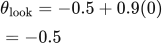 LaTeX:
\theta_{\mathrm{look}}=-0.5+0.9(0)=-0.5LaTeX: g_1=-0.5-(1)=-1.5LaTeX: v_1=0.9(0)-0.1(-1.5)=0.15LaTeX: \theta_1=-0.5+(0.15)=-0.35Step 2: Update 2.
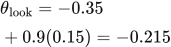 LaTeX:
\theta_{\mathrm{look}}=-0.35+0.9(0.15)=-0.215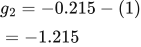 LaTeX:
g_2=-0.215-(1)=-1.215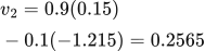 LaTeX:
v_2=0.9(0.15)-0.1(-1.215)=0.2565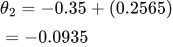 LaTeX:
\theta_2=-0.35+(0.2565)=-0.0935Final parameter after two updates: -0.0935. The lookahead locates the gradient; the new velocity is added to the old actual parameter, not to the lookahead.
AdaGrad
AdaGrad stores a running sum of squared gradients for each parameter. Squaring removes the sign only in this stored total. The unsquared gradient in the numerator still decides the direction of the update.
 LaTeX:
G_t=G_{t-1}+g_t^2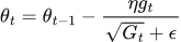 LaTeX:
\theta_t=\theta_{t-1}-\frac{\eta g_t}{\sqrt{G_t}+\epsilon}AdaGrad adds every squared gradient
Definition. AdaGrad is an adaptive first-order optimizer that scales each parameter's update using the inverse square root of the sum of its previous and current squared gradients. Each parameter maintains its own accumulator.
State, effective learning rate and update
For one parameter θ, let gₜ be its current gradient and s₀ = 0:
 LaTeX:
s_t=s_{t-1}+g_t^2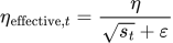 LaTeX:
\eta_{\mathrm{effective},t}=\frac{\eta}{\sqrt{s_t}+\varepsilon} LaTeX:
\theta_t=\theta_{t-1}-\eta_{\mathrm{effective},t}g_ts stores squared-gradient history. Both positive and negative gradients increase this nonnegative sum after squaring. The effective learning rate is the coefficient multiplying the signed gradient; the actual displacement also depends on that gradient's magnitude and sign.
Complete numerical: supplied gradients
Question. Start θ₀ = 1, s₀ = 0, η = 0.1. Given gradients g₁ = 2 and g₂ = 1, perform two AdaGrad updates. Ignore epsilon only for this hand calculation because neither denominator is zero.
Given
θ₀ = 1; initial state(s) = 0; η = 0.1.
Supplied gradients g₁ = 2, g₂ = 1.
ε = 0 for this hand calculation.
To find
Calculate all required states and the parameter after each of two updates.
Formula — which one and why
AdaGrad. Add the new squared gradient to all previous squares. Divide the signed current gradient by the square root of that accumulated magnitude.
G = accumulated squared gradients (also denoted s in some lessons); g = current gradient; η = base learning rate; ε = small stabilizer, set to zero only where the question says so.
LaTeX: G_t=G_{t-1}+g_t^2LaTeX: \theta_t=\theta_{t-1}-\frac{\eta g_t}{\sqrt{G_t}+\epsilon}Yaad rakhne ka cue: Square karo, purane sum mein jodo, root se scale karo.
Solution — step by step
The gradients are supplied by the question. They are not computed from an assumed objective, and g₂ is not replaced by the updated parameter.
Iteration 1 — step 1: update the accumulator.
 LaTeX:
s_1=0+2^2=4Step 2: calculate the effective learning rate.
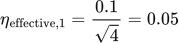 LaTeX:
\eta_{\mathrm{effective},1}=\frac{0.1}{\sqrt4}=0.05Step 3: apply the signed gradient.
 LaTeX:
\theta_1=1-0.05(2)=0.9Iteration 2 — step 1: retain s₁ and add the new squared gradient.
 LaTeX:
s_2=4+1^2=5Step 2: calculate the new coefficient.
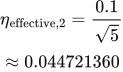 LaTeX:
\eta_{\mathrm{effective},2}=\frac{0.1}{\sqrt5}\approx0.044721360Step 3: update from θ₁.
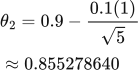 LaTeX:
\theta_2=0.9-\frac{0.1(1)}{\sqrt5}\approx0.855278640Final answer: θ₁ = 0.9 and θ₂ ≈ 0.855279, with accumulators s₁ = 4 and s₂ = 5.
Advantage, limitation and epsilon convention
Coordinate-specific scaling can be useful when some features or gradients occur infrequently. Because s never decreases, its effective learning rate is nonincreasing when η and ε are fixed, and can become too small during prolonged training. The actual displacement magnitude need not decrease monotonically because gₜ also changes.
ε is normally a small positive stabilizer. These notes place it outside the square root. If a question places it inside, use that specified denominator consistently; the two placements are not numerically identical.
Drill 22 AdaGrad variation 1
Question
Question. θ₀ = 1, η = 0.1, supplied successive gradients = [2, 1]. Use AdaGrad for two updates, zero initial accumulators and ε = 0 for this hand calculation.
Answer — step by step
Given
Initial θ₀ = 1; η = 0.1.
Supplied gradients: [2,1].
Initial accumulator(s) = 0; ε = 0 for this nonzero-denominator hand calculation.
To find
Find every stored state needed by the method and the parameter after each of two updates.
Formula — which one and why
AdaGrad. Add the new squared gradient to all previous squares. Divide the signed current gradient by the square root of that accumulated magnitude.
G = accumulated squared gradients (also denoted s in some lessons); g = current gradient; η = base learning rate; ε = small stabilizer, set to zero only where the question says so.
LaTeX: G_t=G_{t-1}+g_t^2LaTeX: \theta_t=\theta_{t-1}-\frac{\eta g_t}{\sqrt{G_t}+\epsilon}Yaad rakhne ka cue: Square karo, purane sum mein jodo, root se scale karo.
Solution — step by step
Symbols and formulas used
θ is the parameter; η is the base learning rate; gₜ is the supplied gradient for update t. The gradients are already given, so no loss differentiation is needed here. Use ε = 0 only as specified in this exercise.
G is a running sum of squared gradients. Squaring removes the sign only inside G; keep the gradient sign in the update numerator. Start G₀ = 0.
LaTeX: G_t=G_{t-1}+g_t^2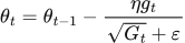 LaTeX:
\theta_t=\theta_{t-1}-\frac{\eta g_t}{\sqrt{G_t}+\varepsilon}Use the supplied gradients in order. Initialize the stated memories to zero. Epsilon is set to zero only for this exercise because every denominator is nonzero. Keep calculator precision until the final result.
Step 1: Iteration 1 with supplied gradient 2.
Add the new squared gradient to all previous squares.
 LaTeX:
G_1=0+(2)^2=4 LaTeX:
\sqrt{G_1}=\sqrt{4}=2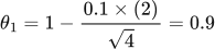 LaTeX:
\theta_1=1-\frac{0.1\times(2)}{\sqrt{4}}=0.9Step 2: Iteration 2 with supplied gradient 1.
Add the new squared gradient to all previous squares.
 LaTeX:
G_2=4+(1)^2=5 LaTeX:
\sqrt{G_2}=\sqrt{5}=2.236067977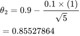 LaTeX:
\theta_2=0.9-\frac{0.1\times(1)}{\sqrt{5}}=0.85527864Drill 23 AdaGrad variation 2
Question
Question. θ₀ = -0.5, η = 0.1, supplied successive gradients = [-1, 2]. Use AdaGrad for two updates, zero initial accumulators and ε = 0 for this hand calculation.
Answer — step by step
Given
Initial θ₀ = −0.5; η = 0.1.
Supplied gradients: [−1,2].
Initial accumulator(s) = 0; ε = 0 for this nonzero-denominator hand calculation.
To find
Find every stored state needed by the method and the parameter after each of two updates.
Formula — which one and why
AdaGrad. Add the new squared gradient to all previous squares. Divide the signed current gradient by the square root of that accumulated magnitude.
G = accumulated squared gradients (also denoted s in some lessons); g = current gradient; η = base learning rate; ε = small stabilizer, set to zero only where the question says so.
LaTeX: G_t=G_{t-1}+g_t^2LaTeX: \theta_t=\theta_{t-1}-\frac{\eta g_t}{\sqrt{G_t}+\epsilon}Yaad rakhne ka cue: Square karo, purane sum mein jodo, root se scale karo.
Solution — step by step
Symbols and formulas used
θ is the parameter; η is the base learning rate; gₜ is the supplied gradient for update t. The gradients are already given, so no loss differentiation is needed here. Use ε = 0 only as specified in this exercise.
G is a running sum of squared gradients. Squaring removes the sign only inside G; keep the gradient sign in the update numerator. Start G₀ = 0.
LaTeX: G_t=G_{t-1}+g_t^2LaTeX: \theta_t=\theta_{t-1}-\frac{\eta g_t}{\sqrt{G_t}+\varepsilon}Use the supplied gradients in order. Initialize the stated memories to zero. Epsilon is set to zero only for this exercise because every denominator is nonzero. Keep calculator precision until the final result.
Step 1: Iteration 1 with supplied gradient -1.
Add the new squared gradient to all previous squares.
 LaTeX:
G_1=0+(-1)^2=1 LaTeX:
\sqrt{G_1}=\sqrt{1}=1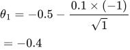 LaTeX:
\theta_1=-0.5-\frac{0.1\times(-1)}{\sqrt{1}}=-0.4Step 2: Iteration 2 with supplied gradient 2.
Add the new squared gradient to all previous squares.
 LaTeX:
G_2=1+(2)^2=5LaTeX: \sqrt{G_2}=\sqrt{5}=2.236067977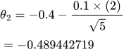 LaTeX:
\theta_2=-0.4-\frac{0.1\times(2)}{\sqrt{5}}=-0.489442719RMSProp
RMSProp remembers a weighted average of squared gradients. With decay 0.9, keep 90% of the old stored value and add 10% of the new squared gradient. Calculate this new stored value before taking its square root and updating the parameter.
 LaTeX:
s_t=\rho s_{t-1}+(1-\rho)g_t^2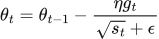 LaTeX:
\theta_t=\theta_{t-1}-\frac{\eta g_t}{\sqrt{s_t}+\epsilon}A moving average remembers the recent past
Definition. An exponentially weighted moving average (EWMA) is a recursively updated estimate in which older observations receive exponentially decreasing weights. Optimizers use it to summarize recent gradients or squared gradients.
 LaTeX:
m_t=\beta m_{t-1}+(1-\beta)g_t,\qquad0\le\beta<1For m₀ = 0, expanding the recurrence gives:
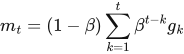 LaTeX:
m_t=(1-\beta)\sum_{k=1}^{t}\beta^{t-k}g_kThe most recent gradient has coefficient 1 − β; a gradient k steps older is discounted by an additional factor βᵏ. Larger β smooths more strongly but responds more slowly to a change in direction. The heuristic averaging horizon is approximately 1/(1 − β); it is not a hard cutoff in the stored history.
Signed gradients versus squared gradients
An average of g contains directional information: positive and negative contributions can cancel. An average of g² estimates the scale through an uncentered second moment and cannot become negative when initialized nonnegatively. Adam tracks both quantities. RMSProp tracks a squared-gradient average in its basic form.
Question. Let β = 0.9, m₀ = 0 and gradients g₁ = 2, g₂ = −1. Find m₁ and m₂.
Given
β = 0.9; initial m₀ = 0.
Gradients in order: g₁ = 2, g₂ = −1.
To find
Find m₁ and m₂, preserving the sign of each gradient.
Formula — which one and why
Exponential moving average. Keep the specified fraction of the old state and add the complementary fraction of the new gradient. This tracks signed direction, so negative gradients can reduce the state.
β (beta) = retained fraction; m = stored average; g = current gradient. m₀ is the initial state.
 LaTeX:
m_t=\beta m_{t-1}+(1-\beta)g_tYaad rakhne ka cue: Beta purani memory rakhta hai; 1−beta naya gradient leta hai.
Solution — step by step
Step 1: find the recent-gradient coefficient.
 LaTeX:
1-0.9=0.1Step 2: retain the old memory for step 1.
 LaTeX:
0.9(0)=0Step 3: weight the first gradient.
 LaTeX:
0.1(2)=0.2Step 4: add to obtain the first memory.
 LaTeX:
m_1=0+0.2=0.2Step 5: retain the first memory for step 2.
 LaTeX:
0.9(0.2)=0.18Step 6: weight the second gradient.
 LaTeX:
0.1(-1)=-0.1Step 7: add to obtain the second memory.
 LaTeX:
m_2=0.18+(-0.1)=0.08Final answer: m₁ = 0.2; m₂ = 0.08.
The second average remains positive although the latest gradient is negative because the previous positive contribution still has weight. If the recurrence is applied to the squared gradients instead, the second state is 0.9(0.4) + 0.1(1) = 0.46. These states have different meanings and are not interchangeable.
RMSProp remembers recent squared gradients
Definition. RMSProp is an adaptive optimizer that normalizes the current gradient by the root of an exponentially weighted moving average of squared gradients. Its decaying history addresses AdaGrad's permanently growing accumulator.
Recurrence and interpretation
Using decay β and zero initial state:
 LaTeX:
s_t=\beta s_{t-1}+(1-\beta)g_t^2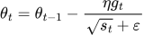 LaTeX:
\theta_t=\theta_{t-1}-\frac{\eta g_t}{\sqrt{s_t}+\varepsilon}β is the fraction of the previous squared-gradient average retained, not a signed velocity. Some papers use ρ for this same decay. The square is applied to the gradient before averaging; the square root is applied to the resulting average in the update.
If recent squared gradients are smaller than the old average, s can decrease. Thus older large gradients do not remain in the denominator with their original weight forever.
Complete numerical: two iterations
Question. θ₀ = 1, s₀ = 0, η = 0.1, β = 0.9; supplied gradients are 2 then 1. Perform two RMSProp updates, with ε = 0 for this hand calculation.
Given
θ₀ = 1; initial state(s) = 0; η = 0.1.
Supplied gradients g₁ = 2, g₂ = 1.
ε = 0 for this hand calculation.
β = 0.9.
To find
Calculate all required states and the parameter after each of two updates.
Formula — which one and why
RMSProp. Use a decaying average of squared gradients, then scale the current gradient by its square root. Old contributions gradually lose influence.
s = squared-gradient average; ρ (rho), sometimes written β, = retained fraction; g = current gradient; η = learning rate; ε = denominator stabilizer.
LaTeX: s_t=\rho s_{t-1}+(1-\rho)g_t^2LaTeX: \theta_t=\theta_{t-1}-\frac{\eta g_t}{\sqrt{s_t}+\epsilon}Yaad rakhne ka cue: Saare purane squares nahi—unki fading average.
Solution — step by step
Iteration 1 — step 1: calculate the squared-gradient average.
 LaTeX:
s_1=0.9(0)+0.1(2^2)=0.4Step 2: calculate the denominator and signed correction.
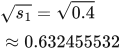 LaTeX:
\sqrt{s_1}=\sqrt{0.4}\approx0.632455532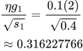 LaTeX:
\frac{\eta g_1}{\sqrt{s_1}}=\frac{0.1(2)}{\sqrt{0.4}}\approx0.316227766Step 3: update the parameter.
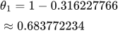 LaTeX:
\theta_1=1-0.316227766\approx0.683772234Iteration 2 — step 1: use s₁, not the original zero state.
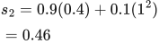 LaTeX:
s_2=0.9(0.4)+0.1(1^2)=0.46Step 2: calculate the denominator and signed correction.
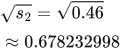 LaTeX:
\sqrt{s_2}=\sqrt{0.46}\approx0.678232998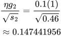 LaTeX:
\frac{\eta g_2}{\sqrt{s_2}}=\frac{0.1(1)}{\sqrt{0.46}}\approx0.147441956Step 3: update from θ₁, retaining calculator precision.
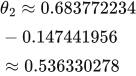 LaTeX:
\theta_2\approx0.683772234-0.147441956\approx0.536330278Final answer: θ₁ ≈ 0.683772 and θ₂ ≈ 0.536330; s₁ = 0.4 and s₂ = 0.46.
Comparison with AdaGrad and Adam
AdaGrad stores an unweighted cumulative sum; RMSProp stores a decaying average. Basic RMSProp has no separate first-moment average and no Adam-style bias correction. With zero initialization, the early RMSProp state can therefore be much smaller than the first squared gradient, which explains the relatively large first correction in this example. The method still requires appropriate learning-rate and decay choices; adaptive scaling does not guarantee convergence to a global optimum.
Drill 24 RMSProp variation 1
Question
Question. θ₀ = 1, η = 0.1, supplied successive gradients = [2, 1]. Use RMSProp for two updates, zero initial accumulators and ε = 0 for this hand calculation. Use ρ = 0.9.
Answer — step by step
Given
Initial θ₀ = 1; η = 0.1.
Supplied gradients: [2,1].
Initial accumulator(s) = 0; ε = 0 for this nonzero-denominator hand calculation.
ρ = 0.9.
To find
Find every stored state needed by the method and the parameter after each of two updates.
Formula — which one and why
RMSProp. Use a decaying average of squared gradients, then scale the current gradient by its square root. Old contributions gradually lose influence.
s = squared-gradient average; ρ (rho), sometimes written β, = retained fraction; g = current gradient; η = learning rate; ε = denominator stabilizer.
LaTeX: s_t=\rho s_{t-1}+(1-\rho)g_t^2LaTeX: \theta_t=\theta_{t-1}-\frac{\eta g_t}{\sqrt{s_t}+\epsilon}Yaad rakhne ka cue: Saare purane squares nahi—unki fading average.
Solution — step by step
Symbols and formulas used
θ is the parameter; η is the base learning rate; gₜ is the supplied gradient for update t. The gradients are already given, so no loss differentiation is needed here. Use ε = 0 only as specified in this exercise.
s is a moving average of squared gradients. ρ = 0.9 retains 90% of the old state; 1 − ρ = 0.1 supplies 10% of the new square. Start s₀ = 0.
LaTeX: s_t=\rho s_{t-1}+(1-\rho)g_t^2LaTeX: \theta_t=\theta_{t-1}-\frac{\eta g_t}{\sqrt{s_t}+\varepsilon}Use the supplied gradients in order. Initialize the stated memories to zero. Epsilon is set to zero only for this exercise because every denominator is nonzero. Keep calculator precision until the final result.
Step 1: Iteration 1 with supplied gradient 2.
Keep 90 percent of the old squared-gradient memory; add 10 percent of the new square.
 LaTeX:
s_1=0.9(0)+0.1(2)^2=0.4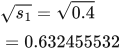 LaTeX:
\sqrt{s_1}=\sqrt{0.4}=0.632455532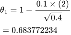 LaTeX:
\theta_1=1-\frac{0.1\times(2)}{\sqrt{0.4}}=0.683772234Step 2: Iteration 2 with supplied gradient 1.
Keep 90 percent of the old squared-gradient memory; add 10 percent of the new square.
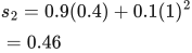 LaTeX:
s_2=0.9(0.4)+0.1(1)^2=0.46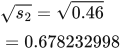 LaTeX:
\sqrt{s_2}=\sqrt{0.46}=0.678232998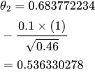 LaTeX:
\theta_2=0.683772234-\frac{0.1\times(1)}{\sqrt{0.46}}=0.536330278Drill 25 RMSProp variation 2
Question
Question. θ₀ = -0.5, η = 0.1, supplied successive gradients = [-1, 2]. Use RMSProp for two updates, zero initial accumulators and ε = 0 for this hand calculation. Use ρ = 0.9.
Answer — step by step
Given
Initial θ₀ = −0.5; η = 0.1.
Supplied gradients: [−1,2].
Initial accumulator(s) = 0; ε = 0 for this nonzero-denominator hand calculation.
ρ = 0.9.
To find
Find every stored state needed by the method and the parameter after each of two updates.
Formula — which one and why
RMSProp. Use a decaying average of squared gradients, then scale the current gradient by its square root. Old contributions gradually lose influence.
s = squared-gradient average; ρ (rho), sometimes written β, = retained fraction; g = current gradient; η = learning rate; ε = denominator stabilizer.
LaTeX: s_t=\rho s_{t-1}+(1-\rho)g_t^2LaTeX: \theta_t=\theta_{t-1}-\frac{\eta g_t}{\sqrt{s_t}+\epsilon}Yaad rakhne ka cue: Saare purane squares nahi—unki fading average.
Solution — step by step
Symbols and formulas used
θ is the parameter; η is the base learning rate; gₜ is the supplied gradient for update t. The gradients are already given, so no loss differentiation is needed here. Use ε = 0 only as specified in this exercise.
s is a moving average of squared gradients. ρ = 0.9 retains 90% of the old state; 1 − ρ = 0.1 supplies 10% of the new square. Start s₀ = 0.
LaTeX: s_t=\rho s_{t-1}+(1-\rho)g_t^2LaTeX: \theta_t=\theta_{t-1}-\frac{\eta g_t}{\sqrt{s_t}+\varepsilon}Use the supplied gradients in order. Initialize the stated memories to zero. Epsilon is set to zero only for this exercise because every denominator is nonzero. Keep calculator precision until the final result.
Step 1: Iteration 1 with supplied gradient -1.
Keep 90 percent of the old squared-gradient memory; add 10 percent of the new square.
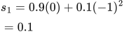 LaTeX:
s_1=0.9(0)+0.1(-1)^2=0.1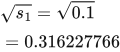 LaTeX:
\sqrt{s_1}=\sqrt{0.1}=0.316227766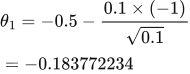 LaTeX:
\theta_1=-0.5-\frac{0.1\times(-1)}{\sqrt{0.1}}=-0.183772234Step 2: Iteration 2 with supplied gradient 2.
Keep 90 percent of the old squared-gradient memory; add 10 percent of the new square.
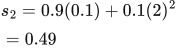 LaTeX:
s_2=0.9(0.1)+0.1(2)^2=0.49 LaTeX:
\sqrt{s_2}=\sqrt{0.49}=0.7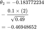 LaTeX:
\theta_2=-0.183772234-\frac{0.1\times(2)}{\sqrt{0.49}}=-0.46948652Adam: both memories
Adam keeps two separate running averages. The first remembers signed gradients and can be negative. The second remembers squared gradients and is nonnegative. These stored averages are not weights, and they are not extra gradients to multiply together.
 LaTeX:
m_t=\beta_1m_{t-1}+(1-\beta_1)g_t LaTeX:
v_t=\beta_2v_{t-1}+(1-\beta_2)g_t^2Optimizer notation: old value, memory, new value
1. A parameter and a stored state are different
θ is the parameter we want to learn. A memory such as v, s or m helps an optimizer decide how to change θ; it is not a second prediction. Each trainable parameter usually has its own corresponding memory entries.
At time t = 0, the problem supplies starting values. At update t = 1, read the old values, calculate the current gradient and new memory, then calculate the new parameter. At update t = 2, use the results of update 1 as the old values.
2. A supplied gradient versus a supplied objective
If the question says gradients are 2 and −1, use those values in order. If it instead gives J(θ) = θ², first differentiate to get g(θ) = 2θ. Recalculate g using the current parameter at each iteration. Nesterov evaluates at its lookahead point instead.
For θ₀ = 1 and η = 0.1 with ordinary GD, g₁ = 2 and θ₁ = 0.8. The next gradient is 2 × 0.8 = 1.6, not the old value 2. Therefore θ₂ = 0.8 − 0.1 × 1.6 = 0.64.
3. A squared gradient keeps size and loses sign
Both 2² and (−2)² equal 4. Squared-gradient memory tells us about scale. The signed numerator still decides the update direction. Never replace the gradient in every part of an optimizer by its square.
4. Square root and epsilon belong to the denominator
If s = 4 and ε = 0.01, the denominator √s + ε is 2 + 0.01 = 2.01. It is different from √(s + ε), which is √4.01. Use the placement specified by the formula. Small ε keeps a zero accumulator from causing division by zero.
5. A table prevents mixing iterations
Write one row per iteration. Ordinary GD needs current θ, gradient and new θ. Momentum adds old and new velocity. Adam adds both memories and their corrected values. Complete a row before starting the next; otherwise a new value from iteration 2 may accidentally be used inside iteration 1.
The worked examples below use this exact order, with every state shown.
Adam remembers both direction and squared size
Definition. Adam, or adaptive moment estimation, uses bias-corrected exponentially weighted estimates of the first moment and the uncentered second moment of gradients to calculate parameter-specific updates.
What the two states represent
| State or coefficient | Meaning |
|---|---|
| mₜ | Moving average of signed gradients; retains directional information |
| sₜ | Moving average of squared gradients; estimates their uncentered second moment |
| β₁ | Decay coefficient for the first-moment estimate |
| β₂ | Decay coefficient for the second-moment estimate |
| t | Update number, starting at 1 for the first update |
| η and ε | Base learning rate and small denominator stabilizer |
The second moment is not the variance: it averages g² without subtracting a mean. Both states start at zero unless specified otherwise. These notes use s throughout this lesson; texts that use v for Adam's second moment mean the same state, not momentum's displacement velocity.
Recurrences, bias correction and update
LaTeX: m_t=\beta_1m_{t-1}+(1-\beta_1)g_t LaTeX:
s_t=\beta_2s_{t-1}+(1-\beta_2)g_t^2Zero initialization reduces the total weight initially attached to observed gradients. Divide by the appropriate accumulated observation weight:
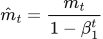 LaTeX:
\hat m_t=\frac{m_t}{1-\beta_1^t} LaTeX:
\hat s_t=\frac{s_t}{1-\beta_2^t}The update uses the corrected signed average in the numerator and the root of the corrected squared-gradient average in the denominator:
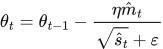 LaTeX:
\theta_t=\theta_{t-1}-\frac{\eta\hat m_t}{\sqrt{\hat s_t}+\varepsilon}The derivation in the next lesson explains why the correction factors contain powers of the iteration number. No additional multiplication by gₜ belongs in this final update: its contribution is already inside mₜ.
Complete numerical: changing gradient magnitude
Question. θ₀ = 1, m₀ = s₀ = 0, η = 0.1, β₁ = 0.9, β₂ = 0.999. Given g₁ = 2 and g₂ = 1, find two Adam updates, neglecting epsilon only in the numerical arithmetic.
Given
θ₀ = 1; initial state(s) = 0; η = 0.1.
Supplied gradients g₁ = 2, g₂ = 1.
ε = 0 for this hand calculation.
β₁ = 0.9; β₂ = 0.999; use bias correction.
To find
Calculate all required states and the parameter after each of two updates.
Formula — which one and why
Adam with bias correction. Keep two states: one averages signed gradients, the other averages squared gradients. Correct their initial bias toward zero before combining them in the parameter update.
m = signed average; s (also written v) = squared average; β₁ and β₂ = retained fractions; t = iteration number. A hat marks a corrected value. Carry raw m and s into the next recurrence.
LaTeX: m_t=\beta_1m_{t-1}+(1-\beta_1)g_tLaTeX: s_t=\beta_2s_{t-1}+(1-\beta_2)g_t^2LaTeX: \hat m_t=\frac{m_t}{1-\beta_1^t}LaTeX: \hat s_t=\frac{s_t}{1-\beta_2^t}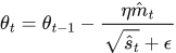 LaTeX:
\theta_t=\theta_{t-1}-\frac{\eta\hat m_t}{\sqrt{\hat s_t}+\epsilon}Yaad rakhne ka cue: Direction memory + square memory; hats lagao, phir update.
Solution — step by step
Iteration 1 — step 1: update the two raw states.
 LaTeX:
m_1=0.9(0)+0.1(2)=0.2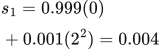 LaTeX:
s_1=0.999(0)+0.001(2^2)=0.004Step 2: correct both states using t = 1.
 LaTeX:
\hat m_1=\frac{0.2}{1-0.9^1}=\frac{0.2}{0.1}=2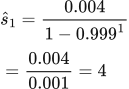 LaTeX:
\hat s_1=\frac{0.004}{1-0.999^1}=\frac{0.004}{0.001}=4Step 3: update the parameter.
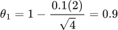 LaTeX:
\theta_1=1-\frac{0.1(2)}{\sqrt4}=0.9Start with the current gradient and the two states saved from the previous iteration.
Carry forward raw states: m = 0.2, s = 0.004. The corrected values are used for this update.
Iteration 2 — step 1: carry forward the raw states m₁ and s₁.
The recurrence uses the raw states 0.2 and 0.004, not the corrected values 2 and 4.
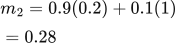 LaTeX:
m_2=0.9(0.2)+0.1(1)=0.28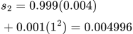 LaTeX:
s_2=0.999(0.004)+0.001(1^2)=0.004996Step 2: correct both states using t = 2.
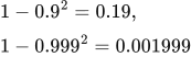 LaTeX:
1-0.9^2=0.19,\qquad1-0.999^2=0.001999 LaTeX:
\hat m_2=\frac{0.28}{0.19}\approx1.473684211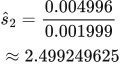 LaTeX:
\hat s_2=\frac{0.004996}{0.001999}\approx2.499249625Step 3: divide the corrected first moment by the corrected root.
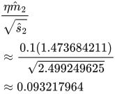 LaTeX:
\frac{\eta\hat m_2}{\sqrt{\hat s_2}}\approx\frac{0.1(1.473684211)}{\sqrt{2.499249625}}\approx0.093217964Step 4: update from θ₁.
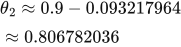 LaTeX:
\theta_2\approx0.9-0.093217964\approx0.806782036Start with the current gradient and the two states saved from the previous iteration.
Carry forward raw states: m = 0.28, s = 0.004996. The corrected values are used for this update.
| State | After iteration 1 | After iteration 2 |
|---|---|---|
| Raw first moment m | 0.2 | 0.28 |
| Raw second moment s | 0.004 | 0.004996 |
| Corrected first moment | 2 | 1.473684211 |
| Corrected second moment | 4 | 2.499249625 |
| Parameter θ | 0.9 | 0.806782036 |
Final answer: θ₁ = 0.9 and θ₂ ≈ 0.806782. Store the raw moments for the next recurrence and use the corrected moments for the current parameter update.
Properties and limitations
Adam combines directional averaging with coordinate-specific scaling, which can be useful with noisy or differently scaled gradients. It requires two state values per parameter in addition to the parameter itself. η, β₁, β₂ and ε remain hyperparameters. Faster reduction of training loss does not establish better generalization, and Adam does not guarantee the global optimum of a general neural-network objective.
Drill 26 Adam variation 1
Question
Question. θ₀ = 1, η = 0.1, supplied successive gradients = [2, 1]. Use Adam for two updates, zero initial accumulators and ε = 0 for this hand calculation. Use β₁ = 0.9, β₂ = 0.999 and bias correction.
Answer — step by step
Given
Initial θ₀ = 1; η = 0.1.
Supplied gradients: [2,1].
Initial accumulator(s) = 0; ε = 0 for this nonzero-denominator hand calculation.
β₁ = 0.9; β₂ = 0.999; use bias correction.
To find
Find every stored state needed by the method and the parameter after each of two updates.
Formula — which one and why
Adam with bias correction. Keep two states: one averages signed gradients, the other averages squared gradients. Correct their initial bias toward zero before combining them in the parameter update.
m = signed average; s (also written v) = squared average; β₁ and β₂ = retained fractions; t = iteration number. A hat marks a corrected value. Carry raw m and s into the next recurrence.
LaTeX: m_t=\beta_1m_{t-1}+(1-\beta_1)g_tLaTeX: s_t=\beta_2s_{t-1}+(1-\beta_2)g_t^2LaTeX: \hat m_t=\frac{m_t}{1-\beta_1^t}LaTeX: \hat s_t=\frac{s_t}{1-\beta_2^t}LaTeX: \theta_t=\theta_{t-1}-\frac{\eta\hat m_t}{\sqrt{\hat s_t}+\epsilon}Yaad rakhne ka cue: Direction memory + square memory; hats lagao, phir update.
Solution — step by step
Symbols and formulas used
θ is the parameter; η is the base learning rate; gₜ is the supplied gradient for update t. The gradients are already given, so no loss differentiation is needed here. Use ε = 0 only as specified in this exercise.
m remembers signed gradients; v remembers squared gradients. The hats mean bias-corrected values, compensating for memories starting at zero. They are not extra powers. Here β₁ = 0.9 and β₂ = 0.999.
LaTeX: m_t=\beta_1m_{t-1}+(1-\beta_1)g_tLaTeX: v_t=\beta_2v_{t-1}+(1-\beta_2)g_t^2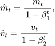 LaTeX:
\hat m_t=\frac{m_t}{1-\beta_1^t},\qquad \hat v_t=\frac{v_t}{1-\beta_2^t}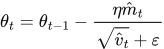 LaTeX:
\theta_t=\theta_{t-1}-\frac{\eta\hat m_t}{\sqrt{\hat v_t}+\varepsilon}Use the supplied gradients in order. Initialize the stated memories to zero. Epsilon is set to zero only for this exercise because every denominator is nonzero. Keep calculator precision until the final result.
Step 1: Iteration 1 with supplied gradient 2.
First calculate the signed-gradient mean m and squared-gradient mean v.
LaTeX: m_1=0.9(0)+0.1(2)=0.2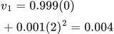 LaTeX:
v_1=0.999(0)+0.001(2)^2=0.004Correct each zero-initialized mean using this iteration number in the power.
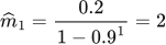 LaTeX:
\widehat m_1=\frac{0.2}{1-0.9^{1}}=2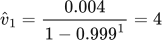 LaTeX:
\widehat v_1=\frac{0.004}{1-0.999^{1}}=4Divide the corrected direction by the corrected root, then subtract the scaled step.
LaTeX: \theta_1=1-\frac{0.1\times(2)}{\sqrt{4}}=0.9Step 2: Iteration 2 with supplied gradient 1.
First calculate the signed-gradient mean m and squared-gradient mean v.
LaTeX: m_2=0.9(0.2)+0.1(1)=0.28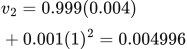 LaTeX:
v_2=0.999(0.004)+0.001(1)^2=0.004996Correct each zero-initialized mean using this iteration number in the power.
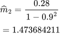 LaTeX:
\widehat m_2=\frac{0.28}{1-0.9^{2}}=1.473684211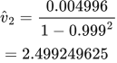 LaTeX:
\widehat v_2=\frac{0.004996}{1-0.999^{2}}=2.499249625Divide the corrected direction by the corrected root, then subtract the scaled step.
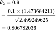 LaTeX:
\theta_2=0.9-\frac{0.1\times(1.473684211)}{\sqrt{2.499249625}}=0.806782036Drill 27 Adam variation 2
Question
Question. θ₀ = -0.5, η = 0.1, supplied successive gradients = [-1, 2]. Use Adam for two updates, zero initial accumulators and ε = 0 for this hand calculation. Use β₁ = 0.9, β₂ = 0.999 and bias correction.
Answer — step by step
Given
Initial θ₀ = −0.5; η = 0.1.
Supplied gradients: [−1,2].
Initial accumulator(s) = 0; ε = 0 for this nonzero-denominator hand calculation.
β₁ = 0.9; β₂ = 0.999; use bias correction.
To find
Find every stored state needed by the method and the parameter after each of two updates.
Formula — which one and why
Adam with bias correction. Keep two states: one averages signed gradients, the other averages squared gradients. Correct their initial bias toward zero before combining them in the parameter update.
m = signed average; s (also written v) = squared average; β₁ and β₂ = retained fractions; t = iteration number. A hat marks a corrected value. Carry raw m and s into the next recurrence.
LaTeX: m_t=\beta_1m_{t-1}+(1-\beta_1)g_tLaTeX: s_t=\beta_2s_{t-1}+(1-\beta_2)g_t^2LaTeX: \hat m_t=\frac{m_t}{1-\beta_1^t}LaTeX: \hat s_t=\frac{s_t}{1-\beta_2^t}LaTeX: \theta_t=\theta_{t-1}-\frac{\eta\hat m_t}{\sqrt{\hat s_t}+\epsilon}Yaad rakhne ka cue: Direction memory + square memory; hats lagao, phir update.
Solution — step by step
Symbols and formulas used
θ is the parameter; η is the base learning rate; gₜ is the supplied gradient for update t. The gradients are already given, so no loss differentiation is needed here. Use ε = 0 only as specified in this exercise.
m remembers signed gradients; v remembers squared gradients. The hats mean bias-corrected values, compensating for memories starting at zero. They are not extra powers. Here β₁ = 0.9 and β₂ = 0.999.
LaTeX: m_t=\beta_1m_{t-1}+(1-\beta_1)g_tLaTeX: v_t=\beta_2v_{t-1}+(1-\beta_2)g_t^2LaTeX: \hat m_t=\frac{m_t}{1-\beta_1^t},\qquad \hat v_t=\frac{v_t}{1-\beta_2^t}LaTeX: \theta_t=\theta_{t-1}-\frac{\eta\hat m_t}{\sqrt{\hat v_t}+\varepsilon}Use the supplied gradients in order. Initialize the stated memories to zero. Epsilon is set to zero only for this exercise because every denominator is nonzero. Keep calculator precision until the final result.
Step 1: Iteration 1 with supplied gradient -1.
First calculate the signed-gradient mean m and squared-gradient mean v.
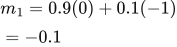 LaTeX:
m_1=0.9(0)+0.1(-1)=-0.1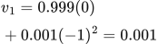 LaTeX:
v_1=0.999(0)+0.001(-1)^2=0.001Correct each zero-initialized mean using this iteration number in the power.
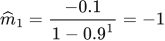 LaTeX:
\widehat m_1=\frac{-0.1}{1-0.9^{1}}=-1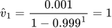 LaTeX:
\widehat v_1=\frac{0.001}{1-0.999^{1}}=1Divide the corrected direction by the corrected root, then subtract the scaled step.
LaTeX: \theta_1=-0.5-\frac{0.1\times(-1)}{\sqrt{1}}=-0.4Step 2: Iteration 2 with supplied gradient 2.
First calculate the signed-gradient mean m and squared-gradient mean v.
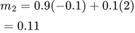 LaTeX:
m_2=0.9(-0.1)+0.1(2)=0.11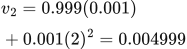 LaTeX:
v_2=0.999(0.001)+0.001(2)^2=0.004999Correct each zero-initialized mean using this iteration number in the power.
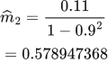 LaTeX:
\widehat m_2=\frac{0.11}{1-0.9^{2}}=0.578947368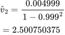 LaTeX:
\widehat v_2=\frac{0.004999}{1-0.999^{2}}=2.500750375Divide the corrected direction by the corrected root, then subtract the scaled step.
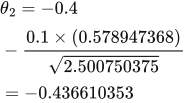 LaTeX:
\theta_2=-0.4-\frac{0.1\times(0.578947368)}{\sqrt{2.500750375}}=-0.436610353Adam: correction and update
Adam starts its two averages at zero. Early averages therefore contain less total weight on observed gradients. Bias correction compensates for that initialization. The power in βᵗ uses the current update number, and both averages must be corrected before the parameter update.
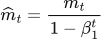 LaTeX:
\widehat m_t=\frac{m_t}{1-\beta_1^t} LaTeX:
\widehat v_t=\frac{v_t}{1-\beta_2^t}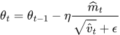 LaTeX:
\theta_t=\theta_{t-1}-\eta\frac{\widehat m_t}{\sqrt{\widehat v_t}+\epsilon}Adam bias correction: why the denominator is one minus beta to a power
Definition. Bias correction compensates for the reduced total observation weight caused by initializing an exponentially weighted accumulator to zero. Under a stationary gradient expectation, it removes the corresponding initialization bias in the moment estimate.
Explanation and working
1. What the moving average actually contains
Adam's signed-gradient memory is m. Starting with m₀ = 0 and β = 0.9, the first average is 90% of zero plus 10% of the first gradient. If g₁ = 2, then m₁ = 0.2. That small value partly reflects the artificial zero initialization.
 LaTeX:
m_1=(1-\beta)g_1At the second step, substitute the first expression into the recurrence:
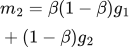 LaTeX:
m_2=\beta(1-\beta)g_1+(1-\beta)g_22. Add the coefficients
After the first step, the total coefficient attached to observed gradients is 1 − β. After two steps it is β(1 − β) + (1 − β). Factor out the common term:
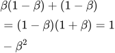 LaTeX:
\beta(1-\beta)+(1-\beta)=(1-\beta)(1+\beta)=1-\beta^2After t steps the coefficients sum to 1 − βᵗ. Dividing the stored average by that quantity removes this zero-start coefficient deficit.
LaTeX: \widehat m_t=\frac{m_t}{1-\beta_1^t}The squared-gradient memory uses its own decay β₂ and the same reasoning:
 LaTeX:
\widehat s_t=\frac{s_t}{1-\beta_2^t}3. A constant-gradient example makes the purpose visible
Let both gradients be 2 and use β₁ = 0.9. The first raw mean is 0.2; the second is 0.9 × 0.2 + 0.1 × 2 = 0.38.
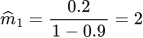 LaTeX:
\widehat m_1=\frac{0.2}{1-0.9}=2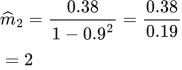 LaTeX:
\widehat m_2=\frac{0.38}{1-0.9^2}=\frac{0.38}{0.19}=2Both corrected values now equal the constant observed gradient. If gradients differ over time, the corrected result is a weighted average, not necessarily the latest gradient.
4. Two betas mean two separate powers
At update 2 with β₁ = 0.9 and β₂ = 0.999, the first correction denominator is 1 − 0.9² = 0.19. The second is 1 − 0.999² = 0.001999. Do not use 0.19 for both memories, and do not keep using the first-step denominators.
5. Correct first, then combine
The parameter update uses the corrected signed mean divided by the square root of the corrected squared mean, plus ε in the stated position. The square root is taken after correcting s. The numerator is not the loss, and no extra multiplication by g follows.
This derivation explains the formula; the following solved Adam examples show the complete arithmetic when gradients change sign or magnitude.
Adam remembers both direction and squared size
Definition. Adam, or adaptive moment estimation, uses bias-corrected exponentially weighted estimates of the first moment and the uncentered second moment of gradients to calculate parameter-specific updates.
What the two states represent
| State or coefficient | Meaning |
|---|---|
| mₜ | Moving average of signed gradients; retains directional information |
| sₜ | Moving average of squared gradients; estimates their uncentered second moment |
| β₁ | Decay coefficient for the first-moment estimate |
| β₂ | Decay coefficient for the second-moment estimate |
| t | Update number, starting at 1 for the first update |
| η and ε | Base learning rate and small denominator stabilizer |
The second moment is not the variance: it averages g² without subtracting a mean. Both states start at zero unless specified otherwise. These notes use s throughout this lesson; texts that use v for Adam's second moment mean the same state, not momentum's displacement velocity.
Recurrences, bias correction and update
LaTeX: m_t=\beta_1m_{t-1}+(1-\beta_1)g_tLaTeX: s_t=\beta_2s_{t-1}+(1-\beta_2)g_t^2Zero initialization reduces the total weight initially attached to observed gradients. Divide by the appropriate accumulated observation weight:
LaTeX: \hat m_t=\frac{m_t}{1-\beta_1^t}LaTeX: \hat s_t=\frac{s_t}{1-\beta_2^t}The update uses the corrected signed average in the numerator and the root of the corrected squared-gradient average in the denominator:
LaTeX: \theta_t=\theta_{t-1}-\frac{\eta\hat m_t}{\sqrt{\hat s_t}+\varepsilon}The derivation in the next lesson explains why the correction factors contain powers of the iteration number. No additional multiplication by gₜ belongs in this final update: its contribution is already inside mₜ.
Complete numerical: changing gradient magnitude
Question. θ₀ = 1, m₀ = s₀ = 0, η = 0.1, β₁ = 0.9, β₂ = 0.999. Given g₁ = 2 and g₂ = 1, find two Adam updates, neglecting epsilon only in the numerical arithmetic.
Given
θ₀ = 1; initial state(s) = 0; η = 0.1.
Supplied gradients g₁ = 2, g₂ = 1.
ε = 0 for this hand calculation.
β₁ = 0.9; β₂ = 0.999; use bias correction.
To find
Calculate all required states and the parameter after each of two updates.
Formula — which one and why
Adam with bias correction. Keep two states: one averages signed gradients, the other averages squared gradients. Correct their initial bias toward zero before combining them in the parameter update.
m = signed average; s (also written v) = squared average; β₁ and β₂ = retained fractions; t = iteration number. A hat marks a corrected value. Carry raw m and s into the next recurrence.
LaTeX: m_t=\beta_1m_{t-1}+(1-\beta_1)g_tLaTeX: s_t=\beta_2s_{t-1}+(1-\beta_2)g_t^2LaTeX: \hat m_t=\frac{m_t}{1-\beta_1^t}LaTeX: \hat s_t=\frac{s_t}{1-\beta_2^t}LaTeX: \theta_t=\theta_{t-1}-\frac{\eta\hat m_t}{\sqrt{\hat s_t}+\epsilon}Yaad rakhne ka cue: Direction memory + square memory; hats lagao, phir update.
Solution — step by step
Iteration 1 — step 1: update the two raw states.
LaTeX: m_1=0.9(0)+0.1(2)=0.2LaTeX: s_1=0.999(0)+0.001(2^2)=0.004Step 2: correct both states using t = 1.
LaTeX: \hat m_1=\frac{0.2}{1-0.9^1}=\frac{0.2}{0.1}=2LaTeX: \hat s_1=\frac{0.004}{1-0.999^1}=\frac{0.004}{0.001}=4Step 3: update the parameter.
LaTeX: \theta_1=1-\frac{0.1(2)}{\sqrt4}=0.9Start with the current gradient and the two states saved from the previous iteration.
Carry forward raw states: m = 0.2, s = 0.004. The corrected values are used for this update.
Iteration 2 — step 1: carry forward the raw states m₁ and s₁.
The recurrence uses the raw states 0.2 and 0.004, not the corrected values 2 and 4.
LaTeX: m_2=0.9(0.2)+0.1(1)=0.28LaTeX: s_2=0.999(0.004)+0.001(1^2)=0.004996Step 2: correct both states using t = 2.
LaTeX: 1-0.9^2=0.19,\qquad1-0.999^2=0.001999LaTeX: \hat m_2=\frac{0.28}{0.19}\approx1.473684211LaTeX: \hat s_2=\frac{0.004996}{0.001999}\approx2.499249625Step 3: divide the corrected first moment by the corrected root.
LaTeX: \frac{\eta\hat m_2}{\sqrt{\hat s_2}}\approx\frac{0.1(1.473684211)}{\sqrt{2.499249625}}\approx0.093217964Step 4: update from θ₁.
LaTeX: \theta_2\approx0.9-0.093217964\approx0.806782036Start with the current gradient and the two states saved from the previous iteration.
Carry forward raw states: m = 0.28, s = 0.004996. The corrected values are used for this update.
| State | After iteration 1 | After iteration 2 |
|---|---|---|
| Raw first moment m | 0.2 | 0.28 |
| Raw second moment s | 0.004 | 0.004996 |
| Corrected first moment | 2 | 1.473684211 |
| Corrected second moment | 4 | 2.499249625 |
| Parameter θ | 0.9 | 0.806782036 |
Final answer: θ₁ = 0.9 and θ₂ ≈ 0.806782. Store the raw moments for the next recurrence and use the corrected moments for the current parameter update.
Properties and limitations
Adam combines directional averaging with coordinate-specific scaling, which can be useful with noisy or differently scaled gradients. It requires two state values per parameter in addition to the parameter itself. η, β₁, β₂ and ε remain hyperparameters. Faster reduction of training loss does not establish better generalization, and Adam does not guarantee the global optimum of a general neural-network objective.
Drill 26 Adam variation 1
Question
Question. θ₀ = 1, η = 0.1, supplied successive gradients = [2, 1]. Use Adam for two updates, zero initial accumulators and ε = 0 for this hand calculation. Use β₁ = 0.9, β₂ = 0.999 and bias correction.
Answer — step by step
Given
Initial θ₀ = 1; η = 0.1.
Supplied gradients: [2,1].
Initial accumulator(s) = 0; ε = 0 for this nonzero-denominator hand calculation.
β₁ = 0.9; β₂ = 0.999; use bias correction.
To find
Find every stored state needed by the method and the parameter after each of two updates.
Formula — which one and why
Adam with bias correction. Keep two states: one averages signed gradients, the other averages squared gradients. Correct their initial bias toward zero before combining them in the parameter update.
m = signed average; s (also written v) = squared average; β₁ and β₂ = retained fractions; t = iteration number. A hat marks a corrected value. Carry raw m and s into the next recurrence.
LaTeX: m_t=\beta_1m_{t-1}+(1-\beta_1)g_tLaTeX: s_t=\beta_2s_{t-1}+(1-\beta_2)g_t^2LaTeX: \hat m_t=\frac{m_t}{1-\beta_1^t}LaTeX: \hat s_t=\frac{s_t}{1-\beta_2^t}LaTeX: \theta_t=\theta_{t-1}-\frac{\eta\hat m_t}{\sqrt{\hat s_t}+\epsilon}Yaad rakhne ka cue: Direction memory + square memory; hats lagao, phir update.
Solution — step by step
Symbols and formulas used
θ is the parameter; η is the base learning rate; gₜ is the supplied gradient for update t. The gradients are already given, so no loss differentiation is needed here. Use ε = 0 only as specified in this exercise.
m remembers signed gradients; v remembers squared gradients. The hats mean bias-corrected values, compensating for memories starting at zero. They are not extra powers. Here β₁ = 0.9 and β₂ = 0.999.
LaTeX: m_t=\beta_1m_{t-1}+(1-\beta_1)g_tLaTeX: v_t=\beta_2v_{t-1}+(1-\beta_2)g_t^2LaTeX: \hat m_t=\frac{m_t}{1-\beta_1^t},\qquad \hat v_t=\frac{v_t}{1-\beta_2^t}LaTeX: \theta_t=\theta_{t-1}-\frac{\eta\hat m_t}{\sqrt{\hat v_t}+\varepsilon}Use the supplied gradients in order. Initialize the stated memories to zero. Epsilon is set to zero only for this exercise because every denominator is nonzero. Keep calculator precision until the final result.
Step 1: Iteration 1 with supplied gradient 2.
First calculate the signed-gradient mean m and squared-gradient mean v.
LaTeX: m_1=0.9(0)+0.1(2)=0.2LaTeX: v_1=0.999(0)+0.001(2)^2=0.004Correct each zero-initialized mean using this iteration number in the power.
LaTeX: \widehat m_1=\frac{0.2}{1-0.9^{1}}=2LaTeX: \widehat v_1=\frac{0.004}{1-0.999^{1}}=4Divide the corrected direction by the corrected root, then subtract the scaled step.
LaTeX: \theta_1=1-\frac{0.1\times(2)}{\sqrt{4}}=0.9Step 2: Iteration 2 with supplied gradient 1.
First calculate the signed-gradient mean m and squared-gradient mean v.
LaTeX: m_2=0.9(0.2)+0.1(1)=0.28LaTeX: v_2=0.999(0.004)+0.001(1)^2=0.004996Correct each zero-initialized mean using this iteration number in the power.
LaTeX: \widehat m_2=\frac{0.28}{1-0.9^{2}}=1.473684211LaTeX: \widehat v_2=\frac{0.004996}{1-0.999^{2}}=2.499249625Divide the corrected direction by the corrected root, then subtract the scaled step.
LaTeX: \theta_2=0.9-\frac{0.1\times(1.473684211)}{\sqrt{2.499249625}}=0.806782036Drill 27 Adam variation 2
Question
Question. θ₀ = -0.5, η = 0.1, supplied successive gradients = [-1, 2]. Use Adam for two updates, zero initial accumulators and ε = 0 for this hand calculation. Use β₁ = 0.9, β₂ = 0.999 and bias correction.
Answer — step by step
Given
Initial θ₀ = −0.5; η = 0.1.
Supplied gradients: [−1,2].
Initial accumulator(s) = 0; ε = 0 for this nonzero-denominator hand calculation.
β₁ = 0.9; β₂ = 0.999; use bias correction.
To find
Find every stored state needed by the method and the parameter after each of two updates.
Formula — which one and why
Adam with bias correction. Keep two states: one averages signed gradients, the other averages squared gradients. Correct their initial bias toward zero before combining them in the parameter update.
m = signed average; s (also written v) = squared average; β₁ and β₂ = retained fractions; t = iteration number. A hat marks a corrected value. Carry raw m and s into the next recurrence.
LaTeX: m_t=\beta_1m_{t-1}+(1-\beta_1)g_tLaTeX: s_t=\beta_2s_{t-1}+(1-\beta_2)g_t^2LaTeX: \hat m_t=\frac{m_t}{1-\beta_1^t}LaTeX: \hat s_t=\frac{s_t}{1-\beta_2^t}LaTeX: \theta_t=\theta_{t-1}-\frac{\eta\hat m_t}{\sqrt{\hat s_t}+\epsilon}Yaad rakhne ka cue: Direction memory + square memory; hats lagao, phir update.
Solution — step by step
Symbols and formulas used
θ is the parameter; η is the base learning rate; gₜ is the supplied gradient for update t. The gradients are already given, so no loss differentiation is needed here. Use ε = 0 only as specified in this exercise.
m remembers signed gradients; v remembers squared gradients. The hats mean bias-corrected values, compensating for memories starting at zero. They are not extra powers. Here β₁ = 0.9 and β₂ = 0.999.
LaTeX: m_t=\beta_1m_{t-1}+(1-\beta_1)g_tLaTeX: v_t=\beta_2v_{t-1}+(1-\beta_2)g_t^2LaTeX: \hat m_t=\frac{m_t}{1-\beta_1^t},\qquad \hat v_t=\frac{v_t}{1-\beta_2^t}LaTeX: \theta_t=\theta_{t-1}-\frac{\eta\hat m_t}{\sqrt{\hat v_t}+\varepsilon}Use the supplied gradients in order. Initialize the stated memories to zero. Epsilon is set to zero only for this exercise because every denominator is nonzero. Keep calculator precision until the final result.
Step 1: Iteration 1 with supplied gradient -1.
First calculate the signed-gradient mean m and squared-gradient mean v.
LaTeX: m_1=0.9(0)+0.1(-1)=-0.1LaTeX: v_1=0.999(0)+0.001(-1)^2=0.001Correct each zero-initialized mean using this iteration number in the power.
LaTeX: \widehat m_1=\frac{-0.1}{1-0.9^{1}}=-1LaTeX: \widehat v_1=\frac{0.001}{1-0.999^{1}}=1Divide the corrected direction by the corrected root, then subtract the scaled step.
LaTeX: \theta_1=-0.5-\frac{0.1\times(-1)}{\sqrt{1}}=-0.4Step 2: Iteration 2 with supplied gradient 2.
First calculate the signed-gradient mean m and squared-gradient mean v.
LaTeX: m_2=0.9(-0.1)+0.1(2)=0.11LaTeX: v_2=0.999(0.001)+0.001(2)^2=0.004999Correct each zero-initialized mean using this iteration number in the power.
LaTeX: \widehat m_2=\frac{0.11}{1-0.9^{2}}=0.578947368LaTeX: \widehat v_2=\frac{0.004999}{1-0.999^{2}}=2.500750375Divide the corrected direction by the corrected root, then subtract the scaled step.
LaTeX: \theta_2=-0.4-\frac{0.1\times(0.578947368)}{\sqrt{2.500750375}}=-0.436610353L1 penalty and update
L1 adds a cost based on the absolute sizes of weights. Its derivative is positive for a positive weight and negative for a negative weight. The optimizer adds this penalty gradient to the data gradient before applying the usual update.
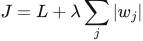 LaTeX:
J=L+\lambda\sum_j|w_j| LaTeX:
w_{new}=w-\eta\left[g_{data}+\lambda\operatorname{sign}(w)\right]Model answer: regularization and the L1–L2 difference
Question
Question. What is regularization? Compare L1 and L2 regularization, including the objective, gradient effect and influence of regularization strength.
Answer — step by step
Regularization restricts or discourages certain fitted solutions to improve generalization. Weight penalties add a cost for parameter size to the training objective. The optimizer must balance fitting the data against that extra cost.
Objectives used in this course
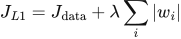 LaTeX:
J_{L1}=J_{\mathrm{data}}+\lambda\sum_i|w_i|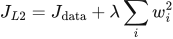 LaTeX:
J_{L2}=J_{\mathrm{data}}+\lambda\sum_iw_i^2Jdata measures prediction error. λ controls the strength of the additional penalty. The sums are over the weights included by the stated question.
| Basis | L1 | L2 |
|---|---|---|
| Quantity penalized | Absolute weight magnitude | Squared weight magnitude |
| Penalty derivative at nonzero w | λ sign(w) | 2λw under the displayed convention |
| Typical effect | Encourages sparse solutions | Smoothly shrinks weight magnitudes |
| Zero weights | Can promote exact zeros with suitable optimization | Usually leaves small nonzero weights |
The total gradient is the data-loss gradient plus the penalty gradient. With w = 2, data gradient 0.3 and λ = 0.1, the displayed L2 penalty adds 2 × 0.1 × 2 = 0.4. The total gradient is 0.7; update using that total.
Increasing λ strengthens the preference for smaller weights. Excessive regularization can prevent learning useful patterns and cause underfitting. L1 is not differentiable at zero, where a subgradient or suitable optimization method is used. If the examination writes λ/2 before the L2 sum, its penalty gradient becomes λw. Derive the factor from the printed objective.
L1 and L2 add a cost for large weights
Definition. Regularization modifies a training objective or learning procedure to constrain the fitted model and improve generalization. L1 and L2 regularization add parameter-norm penalties to the data loss.
Explanation and working
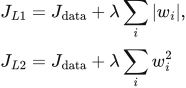 LaTeX:
J_{L1}=J_{\mathrm{data}}+\lambda\sum_i|w_i|,\qquad J_{L2}=J_{\mathrm{data}}+\lambda\sum_iw_i^2Lambda controls how strongly you discourage weight size. L1 encourages sparsity, meaning many weights can become exactly zero under suitable optimization. L2 shrinks weights smoothly and usually leaves small nonzero values. Larger lambda can reduce overfitting, but excessive regularization can underfit.
Question. Data loss = 0.5; weights [2, −1]; λ = 0.1. Compute L1-regularized and L2-regularized objectives using the displayed convention.
Given
Data loss = 0.5; weights = [2,−1]; λ = 0.1.
The L2 convention here has no factor ½.
To find
Find L1/L2 penalties and the two regularized objective values.
Formula — which one and why
L1 penalty and gradient. Add absolute weight magnitudes to penalize large weights. Away from zero, the penalty derivative depends on the weight’s sign.
λ (lambda) = penalty strength; J_data = data loss; sign(w) is +1 for positive and −1 for negative weights. At zero a subgradient convention is needed.
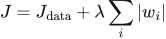 LaTeX:
J=J_{\mathrm{data}}+\lambda\sum_i|w_i| LaTeX:
g_i=g_{\mathrm{data},i}+\lambda\operatorname{sign}(w_i)Yaad rakhne ka cue: L1 absolute values leta hai; gradient mein sign aata hai.
L2 penalty without a factor of one-half. This stated convention multiplies the sum of squares by λ, so differentiating contributes 2λw. Do not use the half-scaled gradient for this objective.
λ = penalty strength; J_data = original data loss; wᵢ = weight i.
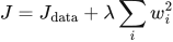 LaTeX:
J=J_{\mathrm{data}}+\lambda\sum_iw_i^2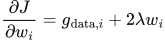 LaTeX:
\frac{\partial J}{\partial w_i}=g_{\mathrm{data},i}+2\lambda w_iYaad rakhne ka cue: Half nahi diya toh L2 derivative mein 2 lambda × weight.
Solution — step by step
Step 1: take absolute values for L1.
 LaTeX:
|2|=2,\qquad|-1|=1Step 2: add the absolute values.
 LaTeX:
2+1=3Step 3: multiply by lambda.
 LaTeX:
0.1(3)=0.3Step 4: add the data loss.
 LaTeX:
J_{L1}=0.5+0.3=0.8Step 5: square both weights for L2.
 LaTeX:
2^2=4,\qquad(-1)^2=1Step 6: add the squares.
 LaTeX:
4+1=5Step 7: multiply by lambda without adding a half.
 LaTeX:
0.1(5)=0.5Step 8: add the data loss.
 LaTeX:
J_{L2}=0.5+0.5=1.0For this L2 convention, the additional gradient is 2 λw. If the objective uses λ/2 times the squared sum, the additional gradient is λw instead. The factor is decided by the stated objective.
L2 gradient update without a half factor
Question. A weight is 2, its data-loss gradient is 0.3, λ = 0.1 and η = 0.01. The objective adds λw². Perform one update.
Given
w = 2; data gradient = 0.3; λ = 0.1; η = 0.01. The penalty has no factor ½.
To find
Penalty gradient, total gradient and updated weight.
Formula — which one and why
The derivative of λw² is 2λw. Add it to the data gradient before applying gradient descent.
λ is penalty strength; η is learning rate; g is the full objective gradient.
 LaTeX:
g_{\mathrm{penalty}}=2\lambda w LaTeX:
g=g_{\mathrm{data}}+g_{\mathrm{penalty}}LaTeX: w_{\mathrm{new}}=w-\eta gYaad rakhne ka cue: Penalty ka gradient data gradient mein jodo, phir update.
Solution — step by step
Step 1: calculate the penalty gradient.
 LaTeX:
2(0.1)(2)=0.4Step 2: add the data gradient.
 LaTeX:
g=0.3+0.4=0.7Step 3: scale by the learning rate.
 LaTeX:
\eta g=0.01(0.7)=0.007Step 4: subtract from the old weight.
 LaTeX:
w_{\mathrm{new}}=2-0.007=1.993Final answer: Updated weight = 1.993. Bias penalties are omitted unless the objective includes them.
Deriving the L2 update
Under the objective written above, the data gradient and penalty gradient add:
 LaTeX:
\nabla_w J=\nabla_w J_{\mathrm{data}}+2\lambda wFor ordinary gradient descent, regrouping the update gives:
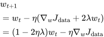 LaTeX:
w_{t+1}=w_t-\eta(\nabla_w J_{\mathrm{data}}+2\lambda w_t)=(1-2\eta\lambda)w_t-\eta\nabla_w J_{\mathrm{data}}This shows the shrinkage associated with this L2 convention. For an objective containing λ‖w‖²/2, replace 2λ by λ. This algebra explains the equivalence to appropriately scaled weight decay for ordinary gradient descent; adding an L2 term inside an adaptive optimizer is generally different from decoupled weight decay.
Drill 29 L1 update on positive and negative weights
Question
Question. w = [−0.5,0.3], data gradients = [0.2,−0.1], λ = 0.1, η = 0.2. Use L1 and ordinary gradient descent away from zero.
Answer — step by step
Given
Old weights = [−0.5,0.3].
Data gradients = [0.2,−0.1]; λ = 0.1; η = 0.2.
To find
Find total gradients and the two updated weights.
Formula — which one and why
L1 penalty and gradient. Add absolute weight magnitudes to penalize large weights. Away from zero, the penalty derivative depends on the weight’s sign.
λ (lambda) = penalty strength; J_data = data loss; sign(w) is +1 for positive and −1 for negative weights. At zero a subgradient convention is needed.
LaTeX: J=J_{\mathrm{data}}+\lambda\sum_i|w_i|LaTeX: g_i=g_{\mathrm{data},i}+\lambda\operatorname{sign}(w_i)Yaad rakhne ka cue: L1 absolute values leta hai; gradient mein sign aata hai.
Gradient descent. Evaluate the gradient at the current parameter, multiply by the learning rate and subtract. If the objective is supplied, differentiate it and recompute the gradient after each update.
θ (theta) = trainable parameter; g = derivative of the stated objective J; η = learning rate; t labels the update number.
LaTeX: g_t=J\prime(\theta_{t-1})LaTeX: \theta_t=\theta_{t-1}-\eta g_tYaad rakhne ka cue: Naya = purana − learning rate × current gradient.
Solution — step by step
Meaning and formula
The supplied data gradient is only one part of the total gradient. L1 adds λ times the sign of the old weight. Sign is −1 for a negative weight and +1 for a positive weight.
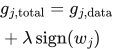 LaTeX:
g_{j,\mathrm{total}}=g_{j,\mathrm{data}}+\lambda\operatorname{sign}(w_j) LaTeX:
w_{j,\mathrm{new}}=w_j-\eta g_{j,\mathrm{total}}Both weights here are nonzero, so the ambiguous derivative of absolute value at zero is not needed.
Step 1: Weight 1: old value −0.5.
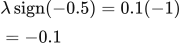 LaTeX:
\lambda\operatorname{sign}(-0.5)=0.1(-1)=-0.1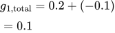 LaTeX:
g_{1,\mathrm{total}}=0.2+(-0.1)=0.1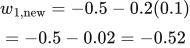 LaTeX:
w_{1,\mathrm{new}}=-0.5-0.2(0.1)=-0.5-0.02=-0.52Step 2: Weight 2: old value 0.3.
 LaTeX:
\lambda\operatorname{sign}(0.3)=0.1(1)=0.1 LaTeX:
g_{2,\mathrm{total}}=-0.1+0.1=0 LaTeX:
w_{2,\mathrm{new}}=0.3-0.2(0)=0.3Final answer: [−0.52, 0.3]. L1's own contribution pulls toward zero, but the combined data-plus-penalty update can move a weight away from zero.
Drill 28 Regularized objective
Question
Question. Data loss = 0.4, w = [−2,1,0.5], λ = 0.1. Calculate L1 objective and L2 objective using (λ/2)Σw².
Answer — step by step
Given
Data loss = 0.4; weights = [−2,1,0.5]; λ = 0.1.
For L2, the question includes the factor ½.
To find
Find each penalty and the total L1/L2 objective.
Formula — which one and why
L1 penalty and gradient. Add absolute weight magnitudes to penalize large weights. Away from zero, the penalty derivative depends on the weight’s sign.
λ (lambda) = penalty strength; J_data = data loss; sign(w) is +1 for positive and −1 for negative weights. At zero a subgradient convention is needed.
LaTeX: J=J_{\mathrm{data}}+\lambda\sum_i|w_i|LaTeX: g_i=g_{\mathrm{data},i}+\lambda\operatorname{sign}(w_i)Yaad rakhne ka cue: L1 absolute values leta hai; gradient mein sign aata hai.
L2 penalty with a factor of one-half. Square each weight, sum and multiply by λ/2. The one-half cancels the factor 2 when differentiating, so the extra gradient is λw.
λ = penalty strength; w = old weight; J_data and g_data = data loss and its gradient.
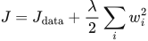 LaTeX:
J=J_{\mathrm{data}}+\frac\lambda2\sum_iw_i^2 LaTeX:
g_i=g_{\mathrm{data},i}+\lambda w_i LaTeX:
w_i^{\mathrm{new}}=w_i-\eta g_iYaad rakhne ka cue: Half wala L2 derivative mein lambda × weight deta hai.
Solution — step by step
Meaning and formulas
The data loss measures prediction error. A regularization penalty adds a cost for large weights. The objective J is the total being minimized. λ sets the strength of the penalty.
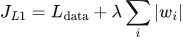 LaTeX:
J_{L1}=L_{\mathrm{data}}+\lambda\sum_i|w_i|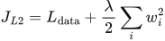 LaTeX:
J_{L2}=L_{\mathrm{data}}+\frac\lambda2\sum_iw_i^2Absolute value means ignore the sign. Squaring means multiply the number by itself. These are different operations.
Step 1: Part A: L1 objective.
 LaTeX:
|-2|=2,\quad |1|=1,\quad |0.5|=0.5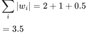 LaTeX:
\sum_i|w_i|=2+1+0.5=3.5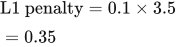 LaTeX:
\text{L1 penalty}=0.1\times3.5=0.35 LaTeX:
J_{L1}=0.4+0.35=0.75Step 2: Part B: L2 objective with the given half.
 LaTeX:
(-2)^2=4,\quad 1^2=1,\quad 0.5^2=0.25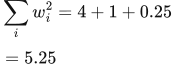 LaTeX:
\sum_iw_i^2=4+1+0.25=5.25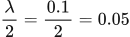 LaTeX:
\frac\lambda2=\frac{0.1}2=0.05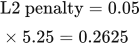 LaTeX:
\text{L2 penalty}=0.05\times5.25=0.2625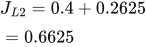 LaTeX:
J_{L2}=0.4+0.2625=0.6625Final answer: L1 objective 0.75; L2 objective 0.6625. These are total objectives, not just penalty values.
Drill 41 Mixed backpropagation and L2
Question
Question. Single linear neuron ŷ = wx, x = 2, w = 0.4, y = 1. Objective J = ½(ŷ−y)²+(λ/2)w², λ = 0.1, η = 0.2. Find loss, gradient, new weight.
Answer — step by step
Given
Prediction ŷ = wx; x = 2; w = 0.4; target y = 1.
Data loss = ½(ŷ−y)²; penalty = (λ/2)w².
λ = 0.1; η = 0.2.
To find
Find total objective, its weight gradient and the new weight.
Formula — which one and why
L2 penalty with a factor of one-half. Square each weight, sum and multiply by λ/2. The one-half cancels the factor 2 when differentiating, so the extra gradient is λw.
λ = penalty strength; w = old weight; J_data and g_data = data loss and its gradient.
LaTeX: J=J_{\mathrm{data}}+\frac\lambda2\sum_iw_i^2LaTeX: g_i=g_{\mathrm{data},i}+\lambda w_iLaTeX: w_i^{\mathrm{new}}=w_i-\eta g_iYaad rakhne ka cue: Half wala L2 derivative mein lambda × weight deta hai.
Gradient descent. Evaluate the gradient at the current parameter, multiply by the learning rate and subtract. If the objective is supplied, differentiate it and recompute the gradient after each update.
θ (theta) = trainable parameter; g = derivative of the stated objective J; η = learning rate; t labels the update number.
LaTeX: g_t=J\prime(\theta_{t-1})LaTeX: \theta_t=\theta_{t-1}-\eta g_tYaad rakhne ka cue: Naya = purana − learning rate × current gradient.
Solution — step by step
Meaning and formulas
This objective contains both prediction error and a weight penalty. Its gradient also has two parts. Compute both at the old weight, add them, then update once.
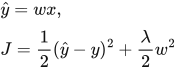 LaTeX:
\hat y=wx,\qquad J=\frac12(\hat y-y)^2+\frac\lambda2w^2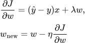 LaTeX:
\frac{\partial J}{\partial w}=(\hat y-y)x+\lambda w,\qquad w_{\mathrm{new}}=w-\eta\frac{\partial J}{\partial w}Step 1: prediction and error
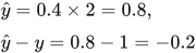 LaTeX:
\hat y=0.4\times2=0.8,\qquad \hat y-y=0.8-1=-0.2Step 2: data loss
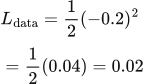 LaTeX:
L_{\mathrm{data}}=\frac12(-0.2)^2=\frac12(0.04)=0.02Step 3: regularization penalty and total objective
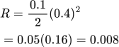 LaTeX:
R=\frac{0.1}{2}(0.4)^2=0.05(0.16)=0.008 LaTeX:
J=0.02+0.008=0.028Step 4: calculate the two gradient contributions
 LaTeX:
g_{\mathrm{data}}=(-0.2)\times2=-0.4 LaTeX:
g_{\mathrm{penalty}}=0.1\times0.4=0.04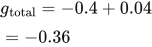 LaTeX:
g_{\mathrm{total}}=-0.4+0.04=-0.36Step 5: update
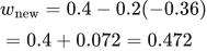 LaTeX:
w_{\mathrm{new}}=0.4-0.2(-0.36)=0.4+0.072=0.472Final answer: total loss 0.028; gradient −0.36; new weight 0.472.
L2 penalty and update with a half
L2 adds a cost based on squared weights. Differentiating a square produces a factor of 2. If the objective includes a half, that half cancels the 2; if it does not, the 2 remains. Read the objective before choosing the gradient.
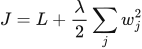 LaTeX:
J=L+\frac\lambda2\sum_jw_j^2 LaTeX:
w_{new}=w-\eta(g_{data}+\lambda w)L1 and L2 add a cost for large weights
Definition. Regularization modifies a training objective or learning procedure to constrain the fitted model and improve generalization. L1 and L2 regularization add parameter-norm penalties to the data loss.
Explanation and working
LaTeX: J_{L1}=J_{\mathrm{data}}+\lambda\sum_i|w_i|,\qquad J_{L2}=J_{\mathrm{data}}+\lambda\sum_iw_i^2Lambda controls how strongly you discourage weight size. L1 encourages sparsity, meaning many weights can become exactly zero under suitable optimization. L2 shrinks weights smoothly and usually leaves small nonzero values. Larger lambda can reduce overfitting, but excessive regularization can underfit.
Question. Data loss = 0.5; weights [2, −1]; λ = 0.1. Compute L1-regularized and L2-regularized objectives using the displayed convention.
Given
Data loss = 0.5; weights = [2,−1]; λ = 0.1.
The L2 convention here has no factor ½.
To find
Find L1/L2 penalties and the two regularized objective values.
Formula — which one and why
L1 penalty and gradient. Add absolute weight magnitudes to penalize large weights. Away from zero, the penalty derivative depends on the weight’s sign.
λ (lambda) = penalty strength; J_data = data loss; sign(w) is +1 for positive and −1 for negative weights. At zero a subgradient convention is needed.
LaTeX: J=J_{\mathrm{data}}+\lambda\sum_i|w_i|LaTeX: g_i=g_{\mathrm{data},i}+\lambda\operatorname{sign}(w_i)Yaad rakhne ka cue: L1 absolute values leta hai; gradient mein sign aata hai.
L2 penalty without a factor of one-half. This stated convention multiplies the sum of squares by λ, so differentiating contributes 2λw. Do not use the half-scaled gradient for this objective.
λ = penalty strength; J_data = original data loss; wᵢ = weight i.
LaTeX: J=J_{\mathrm{data}}+\lambda\sum_iw_i^2LaTeX: \frac{\partial J}{\partial w_i}=g_{\mathrm{data},i}+2\lambda w_iYaad rakhne ka cue: Half nahi diya toh L2 derivative mein 2 lambda × weight.
Solution — step by step
Step 1: take absolute values for L1.
LaTeX: |2|=2,\qquad|-1|=1Step 2: add the absolute values.
LaTeX: 2+1=3Step 3: multiply by lambda.
LaTeX: 0.1(3)=0.3Step 4: add the data loss.
LaTeX: J_{L1}=0.5+0.3=0.8Step 5: square both weights for L2.
LaTeX: 2^2=4,\qquad(-1)^2=1Step 6: add the squares.
LaTeX: 4+1=5Step 7: multiply by lambda without adding a half.
LaTeX: 0.1(5)=0.5Step 8: add the data loss.
LaTeX: J_{L2}=0.5+0.5=1.0For this L2 convention, the additional gradient is 2 λw. If the objective uses λ/2 times the squared sum, the additional gradient is λw instead. The factor is decided by the stated objective.
L2 gradient update without a half factor
Question. A weight is 2, its data-loss gradient is 0.3, λ = 0.1 and η = 0.01. The objective adds λw². Perform one update.
Given
w = 2; data gradient = 0.3; λ = 0.1; η = 0.01. The penalty has no factor ½.
To find
Penalty gradient, total gradient and updated weight.
Formula — which one and why
The derivative of λw² is 2λw. Add it to the data gradient before applying gradient descent.
λ is penalty strength; η is learning rate; g is the full objective gradient.
LaTeX: g_{\mathrm{penalty}}=2\lambda wLaTeX: g=g_{\mathrm{data}}+g_{\mathrm{penalty}}LaTeX: w_{\mathrm{new}}=w-\eta gYaad rakhne ka cue: Penalty ka gradient data gradient mein jodo, phir update.
Solution — step by step
Step 1: calculate the penalty gradient.
LaTeX: 2(0.1)(2)=0.4Step 2: add the data gradient.
LaTeX: g=0.3+0.4=0.7Step 3: scale by the learning rate.
LaTeX: \eta g=0.01(0.7)=0.007Step 4: subtract from the old weight.
LaTeX: w_{\mathrm{new}}=2-0.007=1.993Final answer: Updated weight = 1.993. Bias penalties are omitted unless the objective includes them.
Deriving the L2 update
Under the objective written above, the data gradient and penalty gradient add:
LaTeX: \nabla_w J=\nabla_w J_{\mathrm{data}}+2\lambda wFor ordinary gradient descent, regrouping the update gives:
LaTeX: w_{t+1}=w_t-\eta(\nabla_w J_{\mathrm{data}}+2\lambda w_t)=(1-2\eta\lambda)w_t-\eta\nabla_w J_{\mathrm{data}}This shows the shrinkage associated with this L2 convention. For an objective containing λ‖w‖²/2, replace 2λ by λ. This algebra explains the equivalence to appropriately scaled weight decay for ordinary gradient descent; adding an L2 term inside an adaptive optimizer is generally different from decoupled weight decay.
Drill 30 L2 update
Question
Question. w = [0.5,−0.2], data gradients = [0.1,0.3], λ = 0.2, η = 0.1. Use(λ/2)Σw².
Answer — step by step
Given
Old weights = [0.5,−0.2]; data gradients = [0.1,0.3].
λ = 0.2; η = 0.1; penalty = (λ/2)Σw².
To find
Find penalty gradients, total gradients and updated weights.
Formula — which one and why
L2 penalty with a factor of one-half. Square each weight, sum and multiply by λ/2. The one-half cancels the factor 2 when differentiating, so the extra gradient is λw.
λ = penalty strength; w = old weight; J_data and g_data = data loss and its gradient.
LaTeX: J=J_{\mathrm{data}}+\frac\lambda2\sum_iw_i^2LaTeX: g_i=g_{\mathrm{data},i}+\lambda w_iLaTeX: w_i^{\mathrm{new}}=w_i-\eta g_iYaad rakhne ka cue: Half wala L2 derivative mein lambda × weight deta hai.
Solution — step by step
Formula and its reason
The derivative of (λ/2)w² is λw: the 2 from the square cancels the half. Add that regularization gradient to the given data gradient before updating.
 LaTeX:
g_{j,\mathrm{total}}=g_{j,\mathrm{data}}+\lambda w_jLaTeX: w_{j,\mathrm{new}}=w_j-\eta g_{j,\mathrm{total}}Step 1: Weight 1.
 LaTeX:
\lambda w_1=0.2\times0.5=0.1 LaTeX:
g_{1,\mathrm{total}}=0.1+0.1=0.2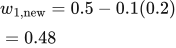 LaTeX:
w_{1,\mathrm{new}}=0.5-0.1(0.2)=0.48Step 2: Weight 2.
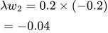 LaTeX:
\lambda w_2=0.2\times(-0.2)=-0.04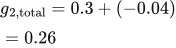 LaTeX:
g_{2,\mathrm{total}}=0.3+(-0.04)=0.26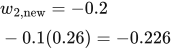 LaTeX:
w_{2,\mathrm{new}}=-0.2-0.1(0.26)=-0.226Final answer: [0.48, −0.226]. The second data gradient dominates the regularization term, explaining why that negative weight becomes more negative.
Drill 28 Regularized objective
Question
Question. Data loss = 0.4, w = [−2,1,0.5], λ = 0.1. Calculate L1 objective and L2 objective using (λ/2)Σw².
Answer — step by step
Given
Data loss = 0.4; weights = [−2,1,0.5]; λ = 0.1.
For L2, the question includes the factor ½.
To find
Find each penalty and the total L1/L2 objective.
Formula — which one and why
L1 penalty and gradient. Add absolute weight magnitudes to penalize large weights. Away from zero, the penalty derivative depends on the weight’s sign.
λ (lambda) = penalty strength; J_data = data loss; sign(w) is +1 for positive and −1 for negative weights. At zero a subgradient convention is needed.
LaTeX: J=J_{\mathrm{data}}+\lambda\sum_i|w_i|LaTeX: g_i=g_{\mathrm{data},i}+\lambda\operatorname{sign}(w_i)Yaad rakhne ka cue: L1 absolute values leta hai; gradient mein sign aata hai.
L2 penalty with a factor of one-half. Square each weight, sum and multiply by λ/2. The one-half cancels the factor 2 when differentiating, so the extra gradient is λw.
λ = penalty strength; w = old weight; J_data and g_data = data loss and its gradient.
LaTeX: J=J_{\mathrm{data}}+\frac\lambda2\sum_iw_i^2LaTeX: g_i=g_{\mathrm{data},i}+\lambda w_iLaTeX: w_i^{\mathrm{new}}=w_i-\eta g_iYaad rakhne ka cue: Half wala L2 derivative mein lambda × weight deta hai.
Solution — step by step
Meaning and formulas
The data loss measures prediction error. A regularization penalty adds a cost for large weights. The objective J is the total being minimized. λ sets the strength of the penalty.
LaTeX: J_{L1}=L_{\mathrm{data}}+\lambda\sum_i|w_i|LaTeX: J_{L2}=L_{\mathrm{data}}+\frac\lambda2\sum_iw_i^2Absolute value means ignore the sign. Squaring means multiply the number by itself. These are different operations.
Step 1: Part A: L1 objective.
LaTeX: |-2|=2,\quad |1|=1,\quad |0.5|=0.5LaTeX: \sum_i|w_i|=2+1+0.5=3.5LaTeX: \text{L1 penalty}=0.1\times3.5=0.35LaTeX: J_{L1}=0.4+0.35=0.75Step 2: Part B: L2 objective with the given half.
LaTeX: (-2)^2=4,\quad 1^2=1,\quad 0.5^2=0.25LaTeX: \sum_iw_i^2=4+1+0.25=5.25LaTeX: \frac\lambda2=\frac{0.1}2=0.05LaTeX: \text{L2 penalty}=0.05\times5.25=0.2625LaTeX: J_{L2}=0.4+0.2625=0.6625Final answer: L1 objective 0.75; L2 objective 0.6625. These are total objectives, not just penalty values.
Drill 41 Mixed backpropagation and L2
Question
Question. Single linear neuron ŷ = wx, x = 2, w = 0.4, y = 1. Objective J = ½(ŷ−y)²+(λ/2)w², λ = 0.1, η = 0.2. Find loss, gradient, new weight.
Answer — step by step
Given
Prediction ŷ = wx; x = 2; w = 0.4; target y = 1.
Data loss = ½(ŷ−y)²; penalty = (λ/2)w².
λ = 0.1; η = 0.2.
To find
Find total objective, its weight gradient and the new weight.
Formula — which one and why
L2 penalty with a factor of one-half. Square each weight, sum and multiply by λ/2. The one-half cancels the factor 2 when differentiating, so the extra gradient is λw.
λ = penalty strength; w = old weight; J_data and g_data = data loss and its gradient.
LaTeX: J=J_{\mathrm{data}}+\frac\lambda2\sum_iw_i^2LaTeX: g_i=g_{\mathrm{data},i}+\lambda w_iLaTeX: w_i^{\mathrm{new}}=w_i-\eta g_iYaad rakhne ka cue: Half wala L2 derivative mein lambda × weight deta hai.
Gradient descent. Evaluate the gradient at the current parameter, multiply by the learning rate and subtract. If the objective is supplied, differentiate it and recompute the gradient after each update.
θ (theta) = trainable parameter; g = derivative of the stated objective J; η = learning rate; t labels the update number.
LaTeX: g_t=J\prime(\theta_{t-1})LaTeX: \theta_t=\theta_{t-1}-\eta g_tYaad rakhne ka cue: Naya = purana − learning rate × current gradient.
Solution — step by step
Meaning and formulas
This objective contains both prediction error and a weight penalty. Its gradient also has two parts. Compute both at the old weight, add them, then update once.
LaTeX: \hat y=wx,\qquad J=\frac12(\hat y-y)^2+\frac\lambda2w^2LaTeX: \frac{\partial J}{\partial w}=(\hat y-y)x+\lambda w,\qquad w_{\mathrm{new}}=w-\eta\frac{\partial J}{\partial w}Step 1: prediction and error
LaTeX: \hat y=0.4\times2=0.8,\qquad \hat y-y=0.8-1=-0.2Step 2: data loss
LaTeX: L_{\mathrm{data}}=\frac12(-0.2)^2=\frac12(0.04)=0.02Step 3: regularization penalty and total objective
LaTeX: R=\frac{0.1}{2}(0.4)^2=0.05(0.16)=0.008LaTeX: J=0.02+0.008=0.028Step 4: calculate the two gradient contributions
LaTeX: g_{\mathrm{data}}=(-0.2)\times2=-0.4LaTeX: g_{\mathrm{penalty}}=0.1\times0.4=0.04LaTeX: g_{\mathrm{total}}=-0.4+0.04=-0.36Step 5: update
LaTeX: w_{\mathrm{new}}=0.4-0.2(-0.36)=0.4+0.072=0.472Final answer: total loss 0.028; gradient −0.36; new weight 0.472.
Inverted dropout
Inverted dropout uses a mask: zero means drop this activation, one means keep it. During training, divide each retained activation by the keep probability. During inference, dropout is disabled and this training-time division is not repeated.
 LaTeX:
q=1-p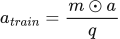 LaTeX:
a_{train}=\frac{m\odot a}{q} LaTeX:
a_{test}=aModel answer: dropout with training and inference explained
Question
Question. Explain dropout as a regularization technique. Distinguish its behavior during training and inference, and explain inverted-dropout scaling.
Answer — step by step
Dropout randomly replaces selected activations by zero during training. It discourages excessive reliance on particular units and their joint activity. The mask changes between training applications; it does not permanently remove neurons or stored weights.
Let p be the probability of dropping an activation and q = 1 − p the probability of keeping it. A mask value m = 1 means keep; m = 0 means drop.
Inverted dropout during training
 LaTeX:
a'=\frac{ma}{q}A kept activation is divided by q and a dropped activation becomes zero. This preserves the activation's expectation over masks.
For a = 3 and q = 0.5, the kept result is 3/0.5 = 6 and the dropped result is 0. Their probability-weighted average is:
 LaTeX:
0.5(6)+0.5(0)=3Inference
Disable dropout and use the ordinary activation. Under inverted dropout there is no further division or multiplication by q at inference. Under the alternative classical convention, training does not rescale kept activations and inference includes the compensating scaling; do not combine the two conventions.
Dropout has no trainable mask parameters. A dropped path contributes zero current data gradient through that activation, although a separately specified weight penalty can still contribute a parameter gradient. Excessive dropout can make optimization or fitting difficult. Choose its rate using validation data.
Dropout removes activations during training
Definition. Dropout is a stochastic regularization method that randomly sets selected unit activations to zero during training. It discourages reliance on specific co-adapted activations; the inference behavior depends on the scaling convention used during training.
Explanation and working
Dropout randomly sets selected activations to zero during training. This discourages dependence on one particular set of neurons. A dropped activation is not a permanently deleted neuron, and dropout does not reduce the model’s stored parameter count.
Let drop probability be p and keep probability be q = 1 − p. A mask entry 1 means keep, 0 means drop. There are two internally consistent scaling conventions.
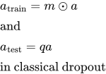 LaTeX:
a_{\mathrm{train}}=m\odot a\quad\text{and}\quad a_{\mathrm{test}}=q a\quad\text{in classical dropout}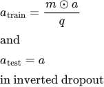 LaTeX:
a_{\mathrm{train}}=\frac{m\odot a}{q}\quad\text{and}\quad a_{\mathrm{test}}=a\quad\text{in inverted dropout}Question. Activations [0.8, −0.4, 0.6, 0.2] have dropout rate 50%. Choose mask [1,0,1,0] and compute outputs.
Given
Activations = [0.8,−0.4,0.6,0.2].
Dropout rate = 50%, so keep probability q = 0.5.
Chosen mask = [1,0,1,0].
To find
Find training outputs under inverted dropout.
Formula — which one and why
Inverted dropout. Multiply by the keep/drop mask, then divide retained activations by the keep probability. This preserves each activation’s expectation over random masks.
aᵢ = original activation; mᵢ is 1 to keep or 0 to drop; q = keep probability = 1−dropout rate. Disable this masking/scaling at inference.
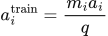 LaTeX:
a_i^{\mathrm{train}}=\frac{m_ia_i}{q} LaTeX:
a_i^{\mathrm{test}}=a_iYaad rakhne ka cue: Mask se keep/drop; kept value ko keep probability se divide.
Solution — step by step
Step 1. q = 1 − 0.5 = 0.5. Apply mask elementwise: [1 × 0.8, 0 × (−0.4), 1 × 0.6, 0 × 0.2] = [0.8,0,0.6,0]. This is the unscaled training output, used by the supplied re-exam key.
Step 2. For inverted dropout, divide the kept outputs by q: [0.8/0.5,0,0.6/0.5,0] = [1.6,0,1.2,0]. Inference then uses the full network without that extra scaling. State the convention in an answer.
Random dropout does not require exactly half the units to disappear in every small layer; each unit is kept or dropped according to the sampling rule. This mask is one possible outcome. If an exam explicitly specifies exactly two dropped units, follow that condition.
Drill 31 Inverted dropout
Question
Question. Activations = [2,−1,0,3], keep probability 0.75, mask = [1,0,1,1]. Find training outputs and explain inference.
Answer — step by step
Given
Activations = [2,−1,0,3].
Keep probability q = 0.75; keep mask = [1,0,1,1].
To find
Find training outputs and state the inference rule.
Formula — which one and why
Inverted dropout. Multiply by the keep/drop mask, then divide retained activations by the keep probability. This preserves each activation’s expectation over random masks.
aᵢ = original activation; mᵢ is 1 to keep or 0 to drop; q = keep probability = 1−dropout rate. Disable this masking/scaling at inference.
LaTeX: a_i^{\mathrm{train}}=\frac{m_ia_i}{q}LaTeX: a_i^{\mathrm{test}}=a_iYaad rakhne ka cue: Mask se keep/drop; kept value ko keep probability se divide.
Solution — step by step
Meaning and formula
The mask entry m is 1 when an activation is kept and 0 when dropped. The keep probability q is 0.75. Inverted dropout divides the kept activations by q during training so that their expected value is preserved.
 LaTeX:
a'_j=\frac{m_j a_j}{q}The multiplication is entry by entry; there is no dot-product sum.
Step 1: apply the mask
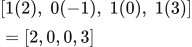 LaTeX:
[1(2),\;0(-1),\;1(0),\;1(3)]=[2,0,0,3]Step 2: divide each result by 0.75
 LaTeX:
a'_1=\frac2{0.75}=2.666666667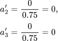 LaTeX:
a'_2=\frac0{0.75}=0,\qquad a'_3=\frac0{0.75}=0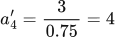 LaTeX:
a'_4=\frac3{0.75}=4Training output = [2.666666667, 0, 0, 4]. A kept activation that was already zero stays zero.
During inference
Disable the random mask and the division. If the incoming activations are the same [2,−1,0,3], they pass through unchanged. The scaling has already been accounted for during training.
Drill 42 Mixed dropout and a momentum update
Question
Question. Hidden activations [1,2], inverted dropout q = 0.5, mask [1,0]. Linear output weights [0.2,0.3], bias 0, target 1, half squared loss. Update only output weights with momentum β = 0.9, old velocity [0.1,−0.1], η = 0.1.
Answer — step by step
Given
Hidden activations = [1,2]; mask = [1,0]; keep probability q = 0.5.
Linear-output weights = [0.2,0.3]; bias = 0; target = 1.
Half squared loss; update only the output weights.
Old signed velocity = [0.1,−0.1]; β = 0.9; η = 0.1.
To find
Find dropped/scaled activations, prediction, gradients, new velocities and new output weights.
Formula — which one and why
Inverted dropout. Multiply by the keep/drop mask, then divide retained activations by the keep probability. This preserves each activation’s expectation over random masks.
aᵢ = original activation; mᵢ is 1 to keep or 0 to drop; q = keep probability = 1−dropout rate. Disable this masking/scaling at inference.
LaTeX: a_i^{\mathrm{train}}=\frac{m_ia_i}{q}LaTeX: a_i^{\mathrm{test}}=a_iYaad rakhne ka cue: Mask se keep/drop; kept value ko keep probability se divide.
Momentum with signed velocity. Combine the retained old displacement with the current downhill correction, then add that signed displacement to the old parameter.
v = signed velocity/displacement; β = momentum coefficient; g = current gradient; η = learning rate. This convention uses +v in the parameter update.
LaTeX: v_t=\beta v_{t-1}-\eta g_tLaTeX: \theta_t=\theta_{t-1}+v_tYaad rakhne ka cue: Pehle velocity banao; phir old parameter mein velocity jodo.
Solution — step by step
Formulas used
Dropout changes the inputs received by the output neuron. Use those changed inputs in both its forward calculation and its weight gradients.
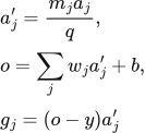 LaTeX:
a'_j=\frac{m_ja_j}{q},\quad o=\sum_jw_ja'_j+b,\quad g_j=(o-y)a'_jThe signed-velocity momentum convention is:
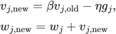 LaTeX:
v_{j,\mathrm{new}}=\beta v_{j,\mathrm{old}}-\eta g_j,\qquad w_{j,\mathrm{new}}=w_j+v_{j,\mathrm{new}}Step 1: apply inverted dropout
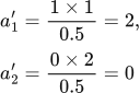 LaTeX:
a'_1=\frac{1\times1}{0.5}=2,\qquad a'_2=\frac{0\times2}{0.5}=0Step 2: prediction and error
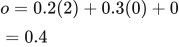 LaTeX:
o=0.2(2)+0.3(0)+0=0.4 LaTeX:
o-y=0.4-1=-0.6Step 3: current weight gradients
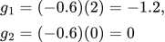 LaTeX:
g_1=(-0.6)(2)=-1.2,\qquad g_2=(-0.6)(0)=0Step 4: remembered movement plus new correction
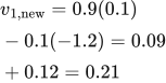 LaTeX:
v_{1,\mathrm{new}}=0.9(0.1)-0.1(-1.2)=0.09+0.12=0.21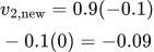 LaTeX:
v_{2,\mathrm{new}}=0.9(-0.1)-0.1(0)=-0.09Step 5: add velocities to old weights
 LaTeX:
w_{1,\mathrm{new}}=0.2+0.21=0.41 LaTeX:
w_{2,\mathrm{new}}=0.3-0.09=0.21Final answer: [0.41, 0.21]. The second weight moves even with zero current gradient because its old momentum is nonzero.
Convolution output dimensions
This formula counts how many legal filter positions fit along one image dimension. Padding adds space at both ends, the kernel occupies K positions, and stride controls how far the next window moves. The floor keeps only complete valid positions.
LaTeX: N_{out}=\left\lfloor\frac{N+2P-K}{S}\right\rfloor+1Reading image shapes before doing CNN arithmetic
Definition. An image or intermediate CNN representation is a tensor indexed by spatial position and channel. This course writes its shape as height × width × channels, excluding the batch dimension.
Explanation and working
Height, width and channels
The shape 4 × 5 × 3 means 4 rows, 5 columns and 3 channels. It contains 4 × 5 × 3 = 60 numbers. A grayscale image commonly has one intensity channel; an RGB image has red, green and blue channels. Intermediate CNN channels are learned feature maps, not necessarily colors.
One position versus the whole map
A filter placed at one location computes one output value. Sliding that same filter over all valid locations creates one feature map. A second filter creates a second feature map. Therefore the number of filters equals the number of output channels.
Why filter depth matches input channels
A 3 × 3 filter applied to a 3-channel input has 3 × 3 × 3 = 27 weights. At one location, it combines 27 input values into one sum. A single bias is then added for that filter. It does not produce three separate output channels just because the input has three channels.
Reading a complete shape calculation
The spatial-size formula computes height and width. It does not compute the channel count.
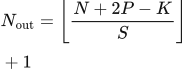 LaTeX:
N_{\mathrm{out}}=\left\lfloor\frac{N+2P-K}{S}\right\rfloor+1N = current input size; P = padding on one side; K = filter size; S = stride. The floor symbol means keep only complete placements. Add one because the initial placement is also an output position.
Shape, parameters and computation are three different counts
Shape counts the arrangement of output values. Parameters count learned weights and biases. Computation counts how many arithmetic operations are performed. Reusing the same filter at 100 positions creates 100 outputs but does not create 100 new sets of weights.
In a multi-layer question, write the output shape of a layer first. That becomes the next layer's input shape. This is why the second convolution uses the first convolution's channel count, not the original image's channel count.
Stride padding and floor
Definition. Stride is the spacing between consecutive kernel positions. Padding extends the input boundary. Together with kernel size and dilation, they determine the spatial dimensions of a convolutional output.
Explanation and working
Stride is how far the filter moves each time. Stride 2 visits starting positions 0, 2, 4 and so on. Padding adds border values, usually zeros. Padding 1 means one new row or column on each side, adding 2 to a spatial dimension.
LaTeX: N_{\mathrm{out}}=\left\lfloor\frac{N+2P-K}{S}\right\rfloor+1N is input size; P is padding per side; K is kernel size; S is stride. Floor means take the greatest integer not above the result:  LaTeX:
\left\lfloor 2.5\right\rfloor = 2. It counts only positions where the entire window fits. The formula assumes dilation 1, the standard setting in these papers. Apply it separately to height and width for rectangular images or kernels.
Why plus one? Even when the kernel exactly fits the image, there is one placement. If N = K, P = 0, S = 1, the formula is 0 + 1 = 1.
Output dimension with a fractional intermediate result
Question. A convolution has input side N = 6, kernel side K = 3, stride S = 2 and padding P = 0. Find its output side.
Given
N = 6; K = 3; S = 2; P = 0; dilation = 1.
To find
The integer output side length.
Formula — which one and why
The formula counts complete kernel placements. Flooring removes an incomplete final placement.
N is input side; P is padding on each side; K is kernel side; S is stride.
LaTeX: N_{\mathrm{out}}=\left\lfloor\frac{N+2P-K}{S}\right\rfloor+1Yaad rakhne ka cue: Padding dono side; stride se divide; floor; phir +1.
Solution — step by step
Step 1: include padding and subtract kernel size.
 LaTeX:
6+2(0)-3=3Step 2: divide by the stride.
 LaTeX:
\frac32=1.5Step 3: take the floor.
 LaTeX:
\lfloor1.5\rfloor=1Step 4: count the first placement.
 LaTeX:
N_{\mathrm{out}}=1+1=2Final answer: Output side = 2; a square input gives a 2 × 2 map per filter.
Padding on both sides
Question. A square convolution input has side 5, kernel side 3, stride 1 and padding 1 on each side. Find the padded-input size and output size.
Given
N = 5; K = 3; S = 1; P = 1 on each side.
To find
Padded input and output dimensions.
Formula — which one and why
Padding adds P entries on each of two opposite sides; the output counts complete kernel placements.
N = unpadded side; K = kernel side; S = stride; P = per-side padding.
 LaTeX:
N_{\mathrm{padded}}=N+2P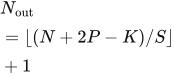 LaTeX:
N_{\mathrm{out}}=\lfloor(N+2P-K)/S\rfloor+1Yaad rakhne ka cue: Padded input aur output ka size alag cheez hain.
Solution — step by step
Step 1: count both padding edges.
 LaTeX:
2P=2(1)=2Step 2: calculate the padded input side.
 LaTeX:
N+2P=5+2=7Step 3: subtract kernel width.
 LaTeX:
7-3=4Step 4: divide by stride and take the floor.
 LaTeX:
\lfloor4/1\rfloor=4Step 5: include the first placement.
 LaTeX:
N_{out}=4+1=5Final answer: Padded input = 7 × 7; output = 5 × 5 per filter.
“Valid” usually means P = 0. For odd K and S = 1, padding (K − 1)/2 preserves the spatial size. For S greater than 1, software “same” padding can be asymmetric and commonly gives ceiling(N/S); do not force the stride-1 rule into that case.
Even-sized kernels: SAME padding is not always symmetric
Definition. A numerical padding value specifies how many entries to add at each boundary. SAME is an output-size convention. At stride 1, SAME preserves height and width; an even-sized kernel can require unequal padding on opposite sides.
For a 2 by 2 kernel at stride 1, preserving the input size requires one padding entry in total per axis, not one on each side. For example, add no row above and one row below, and no column on the left and one on the right. Reversing which side receives the extra entry preserves the output size too, but changes which input cells contribute at each output location; follow the question's convention.
Hinglish cue: P = 1 means dono taraf ek; SAME means output ka size bachao. Dono instructions ko same mat samjho.
Example 1: one entry on every side
Question. A 5 × 5 single-channel input is processed by one 2 × 2 convolution filter. The stride is 1. Exactly one zero is padded on each of the four sides. Find the padded-input size and output size. (Practice: 3 marks)
Given
Input height and width N = 5; kernel size K = 2; stride S = 1; padding P = 1 on each side; dilation = 1; one output filter.
To find
The padded input dimensions and the convolution output dimensions.
Formula — which one and why
The two opposite borders contribute P entries each. The output formula counts complete filter placements after padding.
LaTeX: N_{\mathrm{padded}}=N+2PLaTeX: N_{\mathrm{out}}=\left\lfloor\frac{N+2P-K}{S}\right\rfloor+1N is one input dimension; P is padding on each side; K is kernel size; S is stride. Apply the same calculation separately to height and width. One filter produces one output channel.
Solution — step by step
Step 1: count the two padding borders.
LaTeX: 2P=2(1)=2Step 2: find the padded side length.
 LaTeX:
N_{\mathrm{padded}}=5+2=7The padded input is 7 × 7 × 1.
Step 3: subtract the kernel size.
 LaTeX:
7-2=5Step 4: divide by stride, take the floor and count the first placement.
 LaTeX:
N_{\mathrm{out}}=\left\lfloor\frac{5}{1}\right\rfloor+1=5+1=6Step 5: write height, width and channels.
Both spatial dimensions equal 6. There is one filter, so there is one output channel.
Final answer: padded input = 7 × 7 × 1; output = 6 × 6 × 1. This explicitly specified padding does not implement SAME for this even kernel.
Example 2: preserve the size with SAME padding
Question. The same 5 × 5 single-channel input is processed by one 2 × 2 convolution filter with stride 1 and SAME padding. Find the total padding required along each axis and the output size. Use zero padding above and to the left, with any required extra padding below and to the right. (Practice: 3 marks)
Given
Input side N = 5; kernel side K = 2; stride S = 1; desired output side Nout = 5; dilation = 1; one filter. Padding before the input is 0; padding after the input must be found.
To find
Padding above, below, left and right; padded-input shape; final output shape.
Formula — which one and why
For unequal padding, replace 2P by the sum of the before and after padding. Pbefore and Pafter are the entries added on the two opposite sides of one axis.
 LaTeX:
N_{\mathrm{out}}=\left\lfloor\frac{N+P_{\mathrm{before}}+P_{\mathrm{after}}-K}{S}\right\rfloor+1At stride 1, the quantities are integers. To keep Nout = N, the total padding must equal K − 1.
 LaTeX:
P_{\mathrm{total}}=P_{\mathrm{before}}+P_{\mathrm{after}}=K-1Solution — step by step
Step 1: calculate total padding along the height.
 LaTeX:
P_{\mathrm{total}}=2-1=1Only one extra row in total is needed.
Step 2: place the row using the stated convention.
Padding above = 0; padding below = 1.
Step 3: apply the same calculation to width.
Only one extra column in total is needed. Padding left = 0; padding right = 1.
Step 4: find the padded-input shape.
 LaTeX:
H_{\mathrm{padded}}=5+0+1=6 LaTeX:
W_{\mathrm{padded}}=5+0+1=6The padded input is 6 × 6 × 1.
Step 5: count the output positions along each axis.
 LaTeX:
N_{\mathrm{out}}=\left\lfloor\frac{5+0+1-2}{1}\right\rfloor+1=4+1=5Step 6: include the output channel.
One filter creates one output channel.
Final answer: add 0 above, 1 below, 0 left and 1 right; padded input = 6 × 6 × 1; output = 5 × 5 × 1.
The two questions have the same input and kernel but different padding instructions. Read the stated boundary padding before applying the formula.
Drill 33 Padding stride and channels
Question
Question. Input 31 × 31 × 3; 5 × 5 convolution,8 filters, stride 2, padding 1. Find shape, weights, biases, total.
Answer — step by step
Given
Input shape = 31 × 31 × 3.
Filter size = 5 × 5; number of filters = 8.
Stride S = 2; padding P = 1 per side; one bias per filter.
To find
Find output shape, weights, biases and total parameters.
Formula — which one and why
Convolution/pooling spatial size. Padding adds P positions at both ends. Subtract kernel width to find the last valid start, divide by stride, take the floor and include the initial placement with +1.
N = current height or width; K = kernel/window size; S = stride; P = padding per side. Apply separately to height and width; dilation is 1 here.
LaTeX: N_{\mathrm{out}}=\left\lfloor\frac{N+2P-K}{S}\right\rfloor+1Yaad rakhne ka cue: Input + dono sides ki padding − kernel; stride se divide; floor + 1.
Convolution parameters. Every filter spans all input channels. Count its spatial coefficients across those channels, add one bias and multiply by the number of filters.
K_h,K_w = filter height/width; C_in = input channels; C_out = number of filters and output channels. Spatial output positions reuse these weights.
 LaTeX:
N_w=K_hK_wC_{\mathrm{in}}C_{\mathrm{out}} LaTeX:
N_b=C_{\mathrm{out}} LaTeX:
P=N_w+N_bYaad rakhne ka cue: Filter area × input channels × filters; phir ek bias per filter.
Solution — step by step
Meaning of each given value
The input has height 31, width 31 and 3 channels. K = 5 is the filter width/height; S = 2 is the stride; P = 1 is padding on each side. Eight filters create eight output channels.
Formulas used
LaTeX: N_{\mathrm{out}}=\left\lfloor\frac{N+2P-K}{S}\right\rfloor+1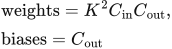 LaTeX:
\text{weights}=K^2C_{\mathrm{in}}C_{\mathrm{out}},\quad \text{biases}=C_{\mathrm{out}}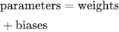 LaTeX:
\text{parameters}=\text{weights}+\text{biases}Step 1: find the output height and width
Padding adds one cell on each side, so the padded width is 31 + 2 × 1 = 33.
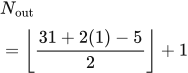 LaTeX:
N_{\mathrm{out}}=\left\lfloor\frac{31+2(1)-5}{2}\right\rfloor+1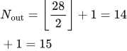 LaTeX:
N_{\mathrm{out}}=\left\lfloor\frac{28}{2}\right\rfloor+1=14+1=15The height uses the same calculation. Output shape = 15 × 15 × 8.
Step 2: count weights in one filter
Each filter covers 5 × 5 positions in each of 3 channels.
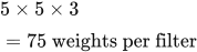 LaTeX:
5\times5\times3=75\text{ weights per filter}Step 3: count all filters and their biases
 LaTeX:
\text{weights}=75\times8=600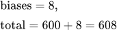 LaTeX:
\text{biases}=8,\qquad \text{total}=600+8=608Final answer: shape 15 × 15 × 8; 600 weights; 8 biases; 608 parameters. The 15 × 15 output locations reuse those weights.
Convolution value
One convolution output is a sum of matched input–kernel products. Move the window and repeat that exact rule for the next output. With several input channels, add contributions from every channel and add the filter bias once.
LaTeX: Y_{ij,o}=\sum_c\sum_u\sum_v K_{uvco}X_{iS+u-P,jS+v-P,c}+b_oOne filter over multiple channels: all contributions go into one cell
Definition. Multi-channel convolution contracts the kernel's spatial and input-channel dimensions to produce one output value per filter at each spatial location. Different filters have independent learned kernels.
Explanation and working
1. Separate spatial size from depth
Imagine a 1 × 1 spatial location with three input channels [2, 5, 1]. A 1 × 1 filter still has one weight for each channel. Suppose its weights are [0.1, −0.2, 0.5] and its bias is 0.3.
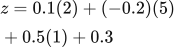 LaTeX:
z=0.1(2)+(-0.2)(5)+0.5(1)+0.3 LaTeX:
z=0.2-1+0.5+0.3=0The three channels contributed to one output value. A single filter creates one output channel, even when its input has several channels.
2. A larger filter has one spatial grid per input channel
A 3 × 3 filter on a three-channel input has three 3 × 3 weight grids, totaling 27 weights. At one output location, calculate the nine products for channel 1, nine for channel 2 and nine for channel 3. Add all 27 products and then add the filter's one bias.
The channel-wise sums are intermediate contributions; do not treat them as three final output channels unless three distinct filters were specified.
3. What changes when there are several filters?
Each filter has its own full-depth weight set and bias. Four filters give four independent sums at each output location, so the result has four channels. The filters all receive the same input depth.
For three input channels and four 3 × 3 filters, parameters are (27 + 1) × 4 = 112. Moving those filters over more image locations reuses these same 112 parameters.
4. One-by-one does not mean one weight
A 1 × 1 convolution with 64 input channels and 16 filters has 64 weights and one bias per filter: (64 + 1) × 16 = 1,040 parameters. It mixes channel information at each spatial position. With 16 outputs it reduces depth from 64 to 16; height and width stay unchanged when stride is 1 and no padding is needed.
This is the channel-reduction idea used by Inception bottlenecks and some residual projections. Spatial kernel size, input depth and output-channel count must all be read separately.
Faculty example: a complete binary-image convolution
Question. Apply the shown 3 × 3 filter to the 5 × 5 image. Use stride 1, no padding and zero bias. Calculate every output value without flipping the filter. (Practice: 5 marks)
Given
Image X = 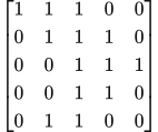 LaTeX:
\begin{bmatrix}1 & 1 & 1 & 0 & 0\\0 & 1 & 1 & 1 & 0\\0 & 0 & 1 & 1 & 1\\0 & 0 & 1 & 1 & 0\\0 & 1 & 1 & 0 & 0\end{bmatrix}.
Filter K =  LaTeX:
\begin{bmatrix}1 & 0 & 1\\0 & 1 & 0\\1 & 0 & 1\end{bmatrix}. These are the values in the Unit 4 lecture example.
To find
The output shape and all nine feature-map values.
Formula — which one and why
The output-size formula counts complete filter placements. At each placement, multiply matching image/filter cells and add the products. A filter entry of zero makes that particular product zero; it does not remove the image cell from the input.
LaTeX: N_{\mathrm{out}}=\left\lfloor\frac{N+2P-K}{S}\right\rfloor+1Here N is input side, K is kernel side, P is padding per side and S is stride. The symbol K in the shape formula is the size 3, whereas the matrix K above contains the filter's coefficients.
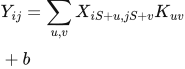 LaTeX:
Y_{ij}=\sum_{u,v}X_{iS+u,jS+v}K_{uv}+bFor this particular filter, only the four corners and the centre of each 3 × 3 window contribute. We can therefore write each sum using those five entries after explaining the four zero products. Below, their order is always top-left, top-right, centre, bottom-left, bottom-right within the current window.
Solution — step by step
Step 1: find the shape. (5 − 3)/1 + 1 = 3. The output is 3 × 3.
Step 2: top-left output, showing all nine products. 1×1 + 1×0 + 1×1 + 0×0 + 1×1 + 1×0 + 0×1 + 0×0 + 1×1 = 1+0+1+0+1+0+0+0+1 = 4.
Step 3: top-middle output. Move the window one column right. Corners and centre are 1,0,1,0,1. Sum = 1+0+1+0+1 = 3.
Step 4: top-right output. Move one more column right. Corners and centre are 1,0,1,1,1. Sum = 1+0+1+1+1 = 4.
Step 5: middle-left output. Return to column 1 and move down one row. Corners and centre are 0,1,0,0,1. Sum = 0+1+0+0+1 = 2.
Step 6: middle-middle output. Corners and centre are 1,1,1,0,1. Sum = 1+1+1+0+1 = 4.
Step 7: middle-right output. Corners and centre are 1,0,1,1,0. Sum = 1+0+1+1+0 = 3.
Step 8: bottom-left output. Corners and centre are 0,1,0,0,1. Sum = 0+1+0+0+1 = 2.
Step 9: bottom-middle output. Corners and centre are 0,1,1,1,0. Sum = 0+1+1+1+0 = 3.
Step 10: bottom-right output. Corners and centre are 1,1,1,1,0. Sum = 1+1+1+1+0 = 4.
Final answer: Y =  LaTeX:
\begin{bmatrix}4 & 3 & 4\\2 & 4 & 3\\2 & 3 & 4\end{bmatrix}. All nine outputs use the same nine filter weights. They do not introduce nine different filters.
Yaad rakho: Window badalta hai; filter ke numbers same rehte hain.
Faculty example: combine three RGB channel sums
Question. At one position, a convolutional filter receives the following red, green and blue 3 × 3 patches and matching kernel slices. Calculate one output value with bias 1. (Practice: 3 marks)
Given
Red patch = 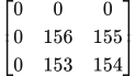 LaTeX:
\begin{bmatrix}0 & 0 & 0\\0 & 156 & 155\\0 & 153 & 154\end{bmatrix}; red kernel = 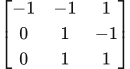 LaTeX:
\begin{bmatrix}-1 & -1 & 1\\0 & 1 & -1\\0 & 1 & 1\end{bmatrix}.
Green patch = 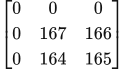 LaTeX:
\begin{bmatrix}0 & 0 & 0\\0 & 167 & 166\\0 & 164 & 165\end{bmatrix}; green kernel = 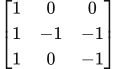 LaTeX:
\begin{bmatrix}1 & 0 & 0\\1 & -1 & -1\\1 & 0 & -1\end{bmatrix}.
Blue patch = 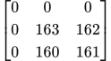 LaTeX:
\begin{bmatrix}0 & 0 & 0\\0 & 163 & 162\\0 & 160 & 161\end{bmatrix}; blue kernel = 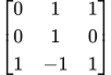 LaTeX:
\begin{bmatrix}0 & 1 & 1\\0 & 1 & 0\\1 & -1 & 1\end{bmatrix}. Bias = 1.
These are three slices of one full-depth filter, not three independent output filters.
To find
The contribution of each input channel and the final scalar output at this position.
Formula — which one and why
Multiply corresponding entries within each channel. Add the three channel sums because this filter spans all input channels. Add its single bias once, after accumulating the channel contributions.
 LaTeX:
z=s_R+s_G+s_B+bThe quantities s_R, s_G and s_B are intermediate weighted sums, not separate final output channels.
Solution — step by step
Step 1: red-channel products. The top row and first column contribute zero. The remaining terms are 156×1 + 155×(−1) + 153×1 + 154×1.
Step 2: red-channel sum. 156 − 155 + 153 + 154 = 308.
Step 3: green-channel products. The remaining patch terms are 167×(−1) + 166×(−1) + 164×0 + 165×(−1).
Step 4: green-channel sum. −167 −166 +0 −165 = −498.
Step 5: blue-channel products. The nonzero-patch terms are 163×1 + 162×0 + 160×(−1) + 161×1.
Step 6: blue-channel sum. 163 +0 −160 +161 = 164.
Step 7: add the channel contributions. 308 −498 +164 = −26.
Step 8: add one filter bias. −26 +1 = −25.
Final answer: The convolution output is −25. If a subsequent ReLU is explicitly requested, that activation produces max(0,−25) = 0. The convolution value and activated value are different stages.
Yaad rakho: Teen channels ka contribution jodo; ek filter ka bias ek baar jodo.
The convolution calculation
Definition. A convolutional layer calculates local weighted sums with a spatially shared kernel and optional bias. Standard deep-learning implementations ordinarily use cross-correlation, without flipping the kernel; examination calculations must follow the stated convention.
Explanation and working
In deep-learning software, the operation normally called convolution is cross-correlation: use the kernel as written, without flipping it. This is the convention in this course’s CNN numericals and the supplied latest answer key. Mathematical convolution would rotate the kernel; state that convention if a question explicitly requests it.
Question. Apply a 2 × 2 kernel Matrix 1 shown below to the 3 × 3 image Matrix 2 shown below, with stride 1, no padding and zero bias.
Given
Input X =  LaTeX:
\begin{bmatrix}1 & 2 & 3\\4 & 5 & 6\\7 & 8 & 9\end{bmatrix}.
Kernel K =  LaTeX:
\begin{bmatrix}1 & 0\\0 & -1\end{bmatrix}.
Stride = 1; padding = 0; bias = 0; no kernel flip.
To find
Find the 2 × 2 output map.
Formula — which one and why
Convolution values. At each valid location, multiply corresponding window and kernel entries, add all products and add the filter bias once. Move by the stated stride and repeat.
X = input; K = kernel; S = stride; b = filter bias; u,v locate a kernel entry. Use the printed kernel without flipping under the stated deep-learning convention.
LaTeX: Y_{ij}=\sum_{u,v}X_{iS+u,jS+v}K_{uv}+bYaad rakhne ka cue: Matching cells multiply; sab products add; bias sirf ek baar.
Solution — step by step
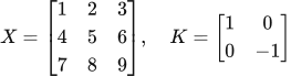 LaTeX:
X=\begin{bmatrix}1&2&3\\4&5&6\\7&8&9\end{bmatrix},\quad K=\begin{bmatrix}1&0\\0&-1\end{bmatrix}Step 1. Top-left window. 1(1) + 2(0) + 4(0) + 5(−1) = 1 − 5 = −4.
Step 2. Move right by one. 2(1) + 3(0) + 5(0) + 6(−1) = 2 − 6 = −4.
Step 3. Move down and return left. 4(1) + 5(0) + 7(0) + 8(−1) = 4 − 8 = −4.
Step 4. Bottom-right window. 5(1) + 6(0) + 8(0) + 9(−1) = 5 − 9 = −4. Output is  LaTeX:
\begin{bmatrix}-4 & -4\\-4 & -4\end{bmatrix}. If ReLU follows, that next layer changes all four entries to zero; do not silently apply it when it was not requested.
Drill 32 Convolution with a negative coefficient
Question
Question. Use the input A and kernel K shown below, stride 1, padding 0. Compute all outputs.
| 1 | 2 | 0 | 1 |
| 0 | 1 | 3 | 2 |
| 2 | 1 | 0 | 1 |
| 1 | 0 | 2 | 3 |
| 1 | −1 |
| 0 | 1 |
Stride 1; P = 0 (no padding).
Answer — step by step
Given
Input A and kernel K are printed with the question.
Stride S = 1; padding P = 0; bias = 0.
Use the kernel without flipping it.
To find
Calculate all nine output cells.
Formula — which one and why
Convolution values. At each valid location, multiply corresponding window and kernel entries, add all products and add the filter bias once. Move by the stated stride and repeat.
X = input; K = kernel; S = stride; b = filter bias; u,v locate a kernel entry. Use the printed kernel without flipping under the stated deep-learning convention.
LaTeX: Y_{ij}=\sum_{u,v}X_{iS+u,jS+v}K_{uv}+bYaad rakhne ka cue: Matching cells multiply; sab products add; bias sirf ek baar.
Solution — step by step
Formulas and the operation we are performing
A filter window produces one output value. Multiply entries at matching positions and add the products. In this deep-learning convention, keep the filter in its printed orientation.
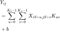 LaTeX:
Y_{ij}=\sum_{u=0}^{K_h-1}\sum_{v=0}^{K_w-1}X_{iS+u,jS+v}K_{uv}+bHere i and j identify an output position; u and v count positions inside its window. S is stride, and b is the filter bias, zero in this question. The equation uses a padded input if padding is present and zero-based indices; the working below labels output positions from 1 for readability.
LaTeX: N_{\mathrm{out}}=\left\lfloor\frac{N+2P-K}{S}\right\rfloor+1N is input width/height, P is padding per side, and K is filter width/height. Floor means take the integer below the result, then add one.
Follow each selected input window below. Matching row colors connect its input cells, kernel coefficients and products; the outlined output cell shows where their sum belongs.
Step 1 shape: 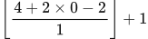 LaTeX:
\left\lfloor\frac{4+2 \times 0-2}{1}\right\rfloor+1 = 3 along each axis. Use the deep-learning cross-correlation convention: do not flip the printed kernel.
Output position (1, 1)
Use this position's input window. Multiply corresponding entries row by row; then add all row totals.
Input rows 1–2, columns 1–2. The window moves 1 cell per output step.
| 1 | 2 | 0 | 1 |
| 0 | 1 | 3 | 2 |
| 2 | 1 | 0 | 1 |
| 1 | 0 | 2 | 3 |
Only the outlined cells belong to this output.
| 1 | −1 |
| 0 | 1 |
Same row and column positions; no matrix multiplication.
| 1 | −2 |
| 0 | 1 |
Each cell is input × matching kernel coefficient.
(−1) + 1 = 0
| 0 | 5 | 1 |
| 0 | −2 | 2 |
| 1 | 3 | 2 |
Output row 1, column 1.
Window row 1.
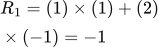 LaTeX:
R_1=(1)\times(1)+(2)\times(-1)=-1Window row 2.
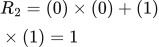 LaTeX:
R_2=(0)\times(0)+(1)\times(1)=1Add the rows to obtain one output cell.
 LaTeX:
Y_{1,1}=(-1)+(1)=0Output position (1, 2)
Use this position's input window. Multiply corresponding entries row by row; then add all row totals.
Input rows 1–2, columns 2–3. The window moves 1 cell per output step.
| 1 | 2 | 0 | 1 |
| 0 | 1 | 3 | 2 |
| 2 | 1 | 0 | 1 |
| 1 | 0 | 2 | 3 |
Only the outlined cells belong to this output.
| 1 | −1 |
| 0 | 1 |
Same row and column positions; no matrix multiplication.
| 2 | 0 |
| 0 | 3 |
Each cell is input × matching kernel coefficient.
2 + 3 = 5
| 0 | 5 | 1 |
| 0 | −2 | 2 |
| 1 | 3 | 2 |
Output row 1, column 2.
Window row 1.
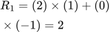 LaTeX:
R_1=(2)\times(1)+(0)\times(-1)=2Window row 2.
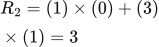 LaTeX:
R_2=(1)\times(0)+(3)\times(1)=3Add the rows to obtain one output cell.
 LaTeX:
Y_{1,2}=(2)+(3)=5Output position (1, 3)
Use this position's input window. Multiply corresponding entries row by row; then add all row totals.
Input rows 1–2, columns 3–4. The window moves 1 cell per output step.
| 1 | 2 | 0 | 1 |
| 0 | 1 | 3 | 2 |
| 2 | 1 | 0 | 1 |
| 1 | 0 | 2 | 3 |
Only the outlined cells belong to this output.
| 1 | −1 |
| 0 | 1 |
Same row and column positions; no matrix multiplication.
| 0 | −1 |
| 0 | 2 |
Each cell is input × matching kernel coefficient.
(−1) + 2 = 1
| 0 | 5 | 1 |
| 0 | −2 | 2 |
| 1 | 3 | 2 |
Output row 1, column 3.
Window row 1.
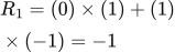 LaTeX:
R_1=(0)\times(1)+(1)\times(-1)=-1Window row 2.
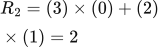 LaTeX:
R_2=(3)\times(0)+(2)\times(1)=2Add the rows to obtain one output cell.
 LaTeX:
Y_{1,3}=(-1)+(2)=1Output position (2, 1)
Use this position's input window. Multiply corresponding entries row by row; then add all row totals.
Input rows 2–3, columns 1–2. The window moves 1 cell per output step.
| 1 | 2 | 0 | 1 |
| 0 | 1 | 3 | 2 |
| 2 | 1 | 0 | 1 |
| 1 | 0 | 2 | 3 |
Only the outlined cells belong to this output.
| 1 | −1 |
| 0 | 1 |
Same row and column positions; no matrix multiplication.
| 0 | −1 |
| 0 | 1 |
Each cell is input × matching kernel coefficient.
(−1) + 1 = 0
| 0 | 5 | 1 |
| 0 | −2 | 2 |
| 1 | 3 | 2 |
Output row 2, column 1.
Window row 1.
LaTeX: R_1=(0)\times(1)+(1)\times(-1)=-1Window row 2.
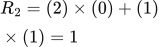 LaTeX:
R_2=(2)\times(0)+(1)\times(1)=1Add the rows to obtain one output cell.
 LaTeX:
Y_{2,1}=(-1)+(1)=0Output position (2, 2)
Use this position's input window. Multiply corresponding entries row by row; then add all row totals.
Input rows 2–3, columns 2–3. The window moves 1 cell per output step.
| 1 | 2 | 0 | 1 |
| 0 | 1 | 3 | 2 |
| 2 | 1 | 0 | 1 |
| 1 | 0 | 2 | 3 |
Only the outlined cells belong to this output.
| 1 | −1 |
| 0 | 1 |
Same row and column positions; no matrix multiplication.
| 1 | −3 |
| 0 | 0 |
Each cell is input × matching kernel coefficient.
(−2) + 0 = −2
| 0 | 5 | 1 |
| 0 | −2 | 2 |
| 1 | 3 | 2 |
Output row 2, column 2.
Window row 1.
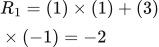 LaTeX:
R_1=(1)\times(1)+(3)\times(-1)=-2Window row 2.
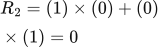 LaTeX:
R_2=(1)\times(0)+(0)\times(1)=0Add the rows to obtain one output cell.
 LaTeX:
Y_{2,2}=(-2)+(0)=-2Output position (2, 3)
Use this position's input window. Multiply corresponding entries row by row; then add all row totals.
Input rows 2–3, columns 3–4. The window moves 1 cell per output step.
| 1 | 2 | 0 | 1 |
| 0 | 1 | 3 | 2 |
| 2 | 1 | 0 | 1 |
| 1 | 0 | 2 | 3 |
Only the outlined cells belong to this output.
| 1 | −1 |
| 0 | 1 |
Same row and column positions; no matrix multiplication.
| 3 | −2 |
| 0 | 1 |
Each cell is input × matching kernel coefficient.
1 + 1 = 2
| 0 | 5 | 1 |
| 0 | −2 | 2 |
| 1 | 3 | 2 |
Output row 2, column 3.
Window row 1.
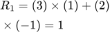 LaTeX:
R_1=(3)\times(1)+(2)\times(-1)=1Window row 2.
LaTeX: R_2=(0)\times(0)+(1)\times(1)=1Add the rows to obtain one output cell.
 LaTeX:
Y_{2,3}=(1)+(1)=2Output position (3, 1)
Use this position's input window. Multiply corresponding entries row by row; then add all row totals.
Input rows 3–4, columns 1–2. The window moves 1 cell per output step.
| 1 | 2 | 0 | 1 |
| 0 | 1 | 3 | 2 |
| 2 | 1 | 0 | 1 |
| 1 | 0 | 2 | 3 |
Only the outlined cells belong to this output.
| 1 | −1 |
| 0 | 1 |
Same row and column positions; no matrix multiplication.
| 2 | −1 |
| 0 | 0 |
Each cell is input × matching kernel coefficient.
1 + 0 = 1
| 0 | 5 | 1 |
| 0 | −2 | 2 |
| 1 | 3 | 2 |
Output row 3, column 1.
Window row 1.
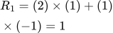 LaTeX:
R_1=(2)\times(1)+(1)\times(-1)=1Window row 2.
LaTeX: R_2=(1)\times(0)+(0)\times(1)=0Add the rows to obtain one output cell.
 LaTeX:
Y_{3,1}=(1)+(0)=1Output position (3, 2)
Use this position's input window. Multiply corresponding entries row by row; then add all row totals.
Input rows 3–4, columns 2–3. The window moves 1 cell per output step.
| 1 | 2 | 0 | 1 |
| 0 | 1 | 3 | 2 |
| 2 | 1 | 0 | 1 |
| 1 | 0 | 2 | 3 |
Only the outlined cells belong to this output.
| 1 | −1 |
| 0 | 1 |
Same row and column positions; no matrix multiplication.
| 1 | 0 |
| 0 | 2 |
Each cell is input × matching kernel coefficient.
1 + 2 = 3
| 0 | 5 | 1 |
| 0 | −2 | 2 |
| 1 | 3 | 2 |
Output row 3, column 2.
Window row 1.
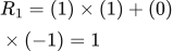 LaTeX:
R_1=(1)\times(1)+(0)\times(-1)=1Window row 2.
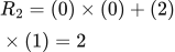 LaTeX:
R_2=(0)\times(0)+(2)\times(1)=2Add the rows to obtain one output cell.
 LaTeX:
Y_{3,2}=(1)+(2)=3Output position (3, 3)
Use this position's input window. Multiply corresponding entries row by row; then add all row totals.
Input rows 3–4, columns 3–4. The window moves 1 cell per output step.
| 1 | 2 | 0 | 1 |
| 0 | 1 | 3 | 2 |
| 2 | 1 | 0 | 1 |
| 1 | 0 | 2 | 3 |
Only the outlined cells belong to this output.
| 1 | −1 |
| 0 | 1 |
Same row and column positions; no matrix multiplication.
| 0 | −1 |
| 0 | 3 |
Each cell is input × matching kernel coefficient.
(−1) + 3 = 2
| 0 | 5 | 1 |
| 0 | −2 | 2 |
| 1 | 3 | 2 |
Output row 3, column 3.
Window row 1.
LaTeX: R_1=(0)\times(1)+(1)\times(-1)=-1Window row 2.
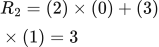 LaTeX:
R_2=(2)\times(0)+(3)\times(1)=3Add the rows to obtain one output cell.
 LaTeX:
Y_{3,3}=(-1)+(3)=2Final output: 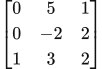 LaTeX:
\begin{bmatrix}0 & 5 & 1\\0 & -2 & 2\\1 & 3 & 2\end{bmatrix}. Each output came from its own complete window; stride changes the next window position, not the multiplication rule.
Drill 40 Mixed convolution pool dense and loss
Question
Question. A is shown below, kernel Matrix 2 shown below, stride 1, valid. Apply ReLU, then 2 × 2 max pool stride 1. Flatten rowwise, use weight vector [0.1,0.2,0.3,0.4], bias 0, sigmoid output, target 1. Find all stages and BCE.
| 1 | 2 | 0 | 1 |
| 0 | 1 | 3 | 2 |
| 2 | 1 | 0 | 1 |
| 1 | 0 | 2 | 3 |
| 1 | 0 |
| 0 | −1 |
Stride 1; P = 0 (no padding).
Answer — step by step
Given
Input A and kernel Matrix 2 are printed with the question.
Conv: stride 1, valid padding; follow with ReLU.
Max pool: 2 × 2, stride 1; flatten row by row.
Dense weights = [0.1,0.2,0.3,0.4]; bias = 0; sigmoid output.
Binary target = 1.
To find
Find convolution, activated map, pooled map, flattened values, prediction and BCE.
Formula — which one and why
Convolution values. At each valid location, multiply corresponding window and kernel entries, add all products and add the filter bias once. Move by the stated stride and repeat.
X = input; K = kernel; S = stride; b = filter bias; u,v locate a kernel entry. Use the printed kernel without flipping under the stated deep-learning convention.
LaTeX: Y_{ij}=\sum_{u,v}X_{iS+u,jS+v}K_{uv}+bYaad rakhne ka cue: Matching cells multiply; sab products add; bias sirf ek baar.
Pooling. Max pooling selects the largest window entry. Average pooling adds its entries and divides by their count. Each channel is pooled separately.
V = current pooling window; n = number of entries in that window. Pooling learns no weights or biases.
 LaTeX:
y_{\max}=\max V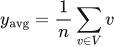 LaTeX:
y_{\mathrm{avg}}=\frac1n\sum_{v\in V}vYaad rakhne ka cue: Max mein biggest; average mein total ÷ window ka count.
Weighted sum and activation. Each input is multiplied by its connection weight. Add these contributions, add the bias once, then apply the stated activation.
xᵢ = input i; wᵢ = its weight; b = bias; z = sum before activation; a = output after activation; f = the specified activation function.
LaTeX: z=\sum_iw_ix_i+bLaTeX: a=f(z)Yaad rakhne ka cue: Input × weight, sabka sum, bias once, phir activation.
Sigmoid and its slope. Use sigmoid when the neuron is specified to squash its preactivation into (0,1). Once its output is known, its derivative needs only output × (1−output).
z = preactivation; p = sigmoid output; e is the exponential base, not a prediction error in this formula.
LaTeX: p=\frac{1}{1+e^{-z}}LaTeX: \frac{dp}{dz}=p(1-p)Yaad rakhne ka cue: Sigmoid output p; uska slope p × (1−p).
Binary cross-entropy. For a binary target, choose the probability of the correct outcome and take its negative natural log. Sigmoid plus BCE has combined logit derivative p−y.
y is 0 or 1; p is the predicted probability of class 1; z is the sigmoid logit. The p−y derivative already includes the sigmoid derivative.
LaTeX: L=-[y\ln p+(1-y)\ln(1-p)]LaTeX: \frac{\partial L}{\partial z}=p-yYaad rakhne ka cue: Binary target 1 ho toh −ln(p); target 0 ho toh −ln(1−p).
Solution — step by step
Formulas and the operation we are performing
A filter window produces one output value. Multiply entries at matching positions and add the products. In this deep-learning convention, keep the filter in its printed orientation.
LaTeX: Y_{ij}=\sum_{u=0}^{K_h-1}\sum_{v=0}^{K_w-1}X_{iS+u,jS+v}K_{uv}+bHere i and j identify an output position; u and v count positions inside its window. S is stride, and b is the filter bias, zero in this question. The equation uses a padded input if padding is present and zero-based indices; the working below labels output positions from 1 for readability.
LaTeX: N_{\mathrm{out}}=\left\lfloor\frac{N+2P-K}{S}\right\rfloor+1N is input width/height, P is padding per side, and K is filter width/height. Floor means take the integer below the result, then add one.
Formulas and meaning
Each 2 × 2 window contains four numbers. Max pooling selects the largest of those four. Average pooling adds all four and divides by 4. Move the window by the given stride after producing one answer.
 LaTeX:
p_{\mathrm{max}}=\max(a_1,a_2,a_3,a_4) LaTeX:
p_{\mathrm{avg}}=\frac{a_1+a_2+a_3+a_4}{4}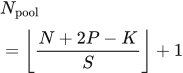 LaTeX:
N_{\mathrm{pool}}=\left\lfloor\frac{N+2P-K}{S}\right\rfloor+1Use the input size at the pooling layer. The output keeps the same channel count.
Completing the network after pooling
Flatten row by row. Multiply the resulting entries by the dense weights and add bias. Apply sigmoid to produce p. For target 1, binary cross-entropy is minus ln(p).
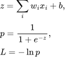 LaTeX:
z=\sum_iw_ix_i+b,\qquad p=\frac1{1+e^{-z}},\qquad L=-\ln pFollow each selected input window below. Matching row colors connect its input cells, kernel coefficients and products; the outlined output cell shows where their sum belongs.
Step 1 shape: LaTeX: \left\lfloor\frac{4+2 \times 0-2}{1}\right\rfloor+1 = 3 along each axis. Use the deep-learning cross-correlation convention: do not flip the printed kernel.
Output position (1, 1)
Use this position's input window. Multiply corresponding entries row by row; then add all row totals.
Input rows 1–2, columns 1–2. The window moves 1 cell per output step.
| 1 | 2 | 0 | 1 |
| 0 | 1 | 3 | 2 |
| 2 | 1 | 0 | 1 |
| 1 | 0 | 2 | 3 |
Only the outlined cells belong to this output.
| 1 | 0 |
| 0 | −1 |
Same row and column positions; no matrix multiplication.
| 1 | 0 |
| 0 | −1 |
Each cell is input × matching kernel coefficient.
1 + (−1) = 0
| 0 | −1 | −2 |
| −1 | 1 | 2 |
| 2 | −1 | −3 |
Output row 1, column 1.
Window row 1.
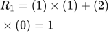 LaTeX:
R_1=(1)\times(1)+(2)\times(0)=1Window row 2.
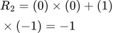 LaTeX:
R_2=(0)\times(0)+(1)\times(-1)=-1Add the rows to obtain one output cell.
 LaTeX:
Y_{1,1}=(1)+(-1)=0Output position (1, 2)
Use this position's input window. Multiply corresponding entries row by row; then add all row totals.
Input rows 1–2, columns 2–3. The window moves 1 cell per output step.
| 1 | 2 | 0 | 1 |
| 0 | 1 | 3 | 2 |
| 2 | 1 | 0 | 1 |
| 1 | 0 | 2 | 3 |
Only the outlined cells belong to this output.
| 1 | 0 |
| 0 | −1 |
Same row and column positions; no matrix multiplication.
| 2 | 0 |
| 0 | −3 |
Each cell is input × matching kernel coefficient.
2 + (−3) = −1
| 0 | −1 | −2 |
| −1 | 1 | 2 |
| 2 | −1 | −3 |
Output row 1, column 2.
Window row 1.
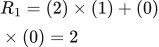 LaTeX:
R_1=(2)\times(1)+(0)\times(0)=2Window row 2.
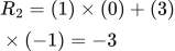 LaTeX:
R_2=(1)\times(0)+(3)\times(-1)=-3Add the rows to obtain one output cell.
 LaTeX:
Y_{1,2}=(2)+(-3)=-1Output position (1, 3)
Use this position's input window. Multiply corresponding entries row by row; then add all row totals.
Input rows 1–2, columns 3–4. The window moves 1 cell per output step.
| 1 | 2 | 0 | 1 |
| 0 | 1 | 3 | 2 |
| 2 | 1 | 0 | 1 |
| 1 | 0 | 2 | 3 |
Only the outlined cells belong to this output.
| 1 | 0 |
| 0 | −1 |
Same row and column positions; no matrix multiplication.
| 0 | 0 |
| 0 | −2 |
Each cell is input × matching kernel coefficient.
0 + (−2) = −2
| 0 | −1 | −2 |
| −1 | 1 | 2 |
| 2 | −1 | −3 |
Output row 1, column 3.
Window row 1.
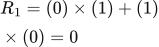 LaTeX:
R_1=(0)\times(1)+(1)\times(0)=0Window row 2.
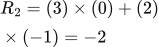 LaTeX:
R_2=(3)\times(0)+(2)\times(-1)=-2Add the rows to obtain one output cell.
 LaTeX:
Y_{1,3}=(0)+(-2)=-2Output position (2, 1)
Use this position's input window. Multiply corresponding entries row by row; then add all row totals.
Input rows 2–3, columns 1–2. The window moves 1 cell per output step.
| 1 | 2 | 0 | 1 |
| 0 | 1 | 3 | 2 |
| 2 | 1 | 0 | 1 |
| 1 | 0 | 2 | 3 |
Only the outlined cells belong to this output.
| 1 | 0 |
| 0 | −1 |
Same row and column positions; no matrix multiplication.
| 0 | 0 |
| 0 | −1 |
Each cell is input × matching kernel coefficient.
0 + (−1) = −1
| 0 | −1 | −2 |
| −1 | 1 | 2 |
| 2 | −1 | −3 |
Output row 2, column 1.
Window row 1.
LaTeX: R_1=(0)\times(1)+(1)\times(0)=0Window row 2.
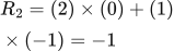 LaTeX:
R_2=(2)\times(0)+(1)\times(-1)=-1Add the rows to obtain one output cell.
 LaTeX:
Y_{2,1}=(0)+(-1)=-1Output position (2, 2)
Use this position's input window. Multiply corresponding entries row by row; then add all row totals.
Input rows 2–3, columns 2–3. The window moves 1 cell per output step.
| 1 | 2 | 0 | 1 |
| 0 | 1 | 3 | 2 |
| 2 | 1 | 0 | 1 |
| 1 | 0 | 2 | 3 |
Only the outlined cells belong to this output.
| 1 | 0 |
| 0 | −1 |
Same row and column positions; no matrix multiplication.
| 1 | 0 |
| 0 | 0 |
Each cell is input × matching kernel coefficient.
1 + 0 = 1
| 0 | −1 | −2 |
| −1 | 1 | 2 |
| 2 | −1 | −3 |
Output row 2, column 2.
Window row 1.
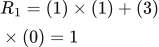 LaTeX:
R_1=(1)\times(1)+(3)\times(0)=1Window row 2.
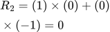 LaTeX:
R_2=(1)\times(0)+(0)\times(-1)=0Add the rows to obtain one output cell.
 LaTeX:
Y_{2,2}=(1)+(0)=1Output position (2, 3)
Use this position's input window. Multiply corresponding entries row by row; then add all row totals.
Input rows 2–3, columns 3–4. The window moves 1 cell per output step.
| 1 | 2 | 0 | 1 |
| 0 | 1 | 3 | 2 |
| 2 | 1 | 0 | 1 |
| 1 | 0 | 2 | 3 |
Only the outlined cells belong to this output.
| 1 | 0 |
| 0 | −1 |
Same row and column positions; no matrix multiplication.
| 3 | 0 |
| 0 | −1 |
Each cell is input × matching kernel coefficient.
3 + (−1) = 2
| 0 | −1 | −2 |
| −1 | 1 | 2 |
| 2 | −1 | −3 |
Output row 2, column 3.
Window row 1.
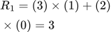 LaTeX:
R_1=(3)\times(1)+(2)\times(0)=3Window row 2.
LaTeX: R_2=(0)\times(0)+(1)\times(-1)=-1Add the rows to obtain one output cell.
 LaTeX:
Y_{2,3}=(3)+(-1)=2Output position (3, 1)
Use this position's input window. Multiply corresponding entries row by row; then add all row totals.
Input rows 3–4, columns 1–2. The window moves 1 cell per output step.
| 1 | 2 | 0 | 1 |
| 0 | 1 | 3 | 2 |
| 2 | 1 | 0 | 1 |
| 1 | 0 | 2 | 3 |
Only the outlined cells belong to this output.
| 1 | 0 |
| 0 | −1 |
Same row and column positions; no matrix multiplication.
| 2 | 0 |
| 0 | 0 |
Each cell is input × matching kernel coefficient.
2 + 0 = 2
| 0 | −1 | −2 |
| −1 | 1 | 2 |
| 2 | −1 | −3 |
Output row 3, column 1.
Window row 1.
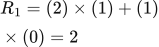 LaTeX:
R_1=(2)\times(1)+(1)\times(0)=2Window row 2.
LaTeX: R_2=(1)\times(0)+(0)\times(-1)=0Add the rows to obtain one output cell.
 LaTeX:
Y_{3,1}=(2)+(0)=2Output position (3, 2)
Use this position's input window. Multiply corresponding entries row by row; then add all row totals.
Input rows 3–4, columns 2–3. The window moves 1 cell per output step.
| 1 | 2 | 0 | 1 |
| 0 | 1 | 3 | 2 |
| 2 | 1 | 0 | 1 |
| 1 | 0 | 2 | 3 |
Only the outlined cells belong to this output.
| 1 | 0 |
| 0 | −1 |
Same row and column positions; no matrix multiplication.
| 1 | 0 |
| 0 | −2 |
Each cell is input × matching kernel coefficient.
1 + (−2) = −1
| 0 | −1 | −2 |
| −1 | 1 | 2 |
| 2 | −1 | −3 |
Output row 3, column 2.
Window row 1.
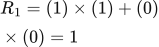 LaTeX:
R_1=(1)\times(1)+(0)\times(0)=1Window row 2.
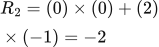 LaTeX:
R_2=(0)\times(0)+(2)\times(-1)=-2Add the rows to obtain one output cell.
 LaTeX:
Y_{3,2}=(1)+(-2)=-1Output position (3, 3)
Use this position's input window. Multiply corresponding entries row by row; then add all row totals.
Input rows 3–4, columns 3–4. The window moves 1 cell per output step.
| 1 | 2 | 0 | 1 |
| 0 | 1 | 3 | 2 |
| 2 | 1 | 0 | 1 |
| 1 | 0 | 2 | 3 |
Only the outlined cells belong to this output.
| 1 | 0 |
| 0 | −1 |
Same row and column positions; no matrix multiplication.
| 0 | 0 |
| 0 | −3 |
Each cell is input × matching kernel coefficient.
0 + (−3) = −3
| 0 | −1 | −2 |
| −1 | 1 | 2 |
| 2 | −1 | −3 |
Output row 3, column 3.
Window row 1.
LaTeX: R_1=(0)\times(1)+(1)\times(0)=0Window row 2.
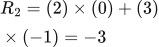 LaTeX:
R_2=(2)\times(0)+(3)\times(-1)=-3Add the rows to obtain one output cell.
 LaTeX:
Y_{3,3}=(0)+(-3)=-3Final output: 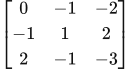 LaTeX:
\begin{bmatrix}0 & -1 & -2\\-1 & 1 & 2\\2 & -1 & -3\end{bmatrix}. Each output came from its own complete window; stride changes the next window position, not the multiplication rule.
ReLU turns negative entries into 0:  LaTeX:
\begin{bmatrix}0 & 0 & 0\\0 & 1 & 2\\2 & 0 & 0\end{bmatrix}.
Shape: 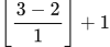 LaTeX:
\left\lfloor\frac{3-2}{1}\right\rfloor+1 = 2 on each axis; channels stay unchanged.
Pooling window (1,1)
Step 1: select the entries.
[0, 0, 0, 1]
Step 2: add all selected entries.
0 + 0 + 0 + 1 = 1
Step 3: divide by the 4 entries in this window.
1/4 = 0.25. Maximum = 1
Pooling window (1,2)
Step 1: select the entries.
[0, 0, 1, 2]
Step 2: add all selected entries.
0 + 0 + 1 + 2 = 3
Step 3: divide by the 4 entries in this window.
3/4 = 0.75. Maximum = 2
Pooling window (2,1)
Step 1: select the entries.
[0, 1, 2, 0]
Step 2: add all selected entries.
0 + 1 + 2 + 0 = 3
Step 3: divide by the 4 entries in this window.
3/4 = 0.75. Maximum = 2
Pooling window (2,2)
Step 1: select the entries.
[1, 2, 0, 0]
Step 2: add all selected entries.
1 + 2 + 0 + 0 = 3
Step 3: divide by the 4 entries in this window.
3/4 = 0.75. Maximum = 2
Average output: 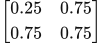 LaTeX:
\begin{bmatrix}0.25 & 0.75\\0.75 & 0.75\end{bmatrix}. Max output:  LaTeX:
\begin{bmatrix}1 & 2\\2 & 2\end{bmatrix}. Pooling normally has zero trainable parameters and reduces spatial dimensions.
Use MAX output and flatten rowwise: [1, 2, 2, 2]. Dense z = 0.1 × 1 + 0.2 × 2 + 0.3 × 2 + 0.4 × 2 = 1.9. p = σ(1.9) = 0.869891526. BCE = −ln(p) = 0.139386758. Average pool values were computed for contrast; the question requires max pool.
Max, min and average pooling
Pooling reduces each window to one value. Max pooling keeps the largest entry; average pooling adds all included entries and divides by their count. Pooling is performed independently in each channel.
LaTeX: y_{\min}=\min(x_1,x_2,x_3,x_4)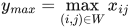 LaTeX:
y_{max}=\max_{(i,j)\in W}x_{ij}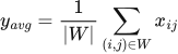 LaTeX:
y_{avg}=\frac1{|W|}\sum_{(i,j)\in W}x_{ij}Pooling needs comparisons or averages
Definition. Pooling is a local aggregation operation that summarizes each spatial window, usually independently per channel. Max pooling selects the largest value; average pooling calculates a mean. Standard pooling has no learned weights or biases.
Explanation and working
Max pooling selects the largest value inside each window. Average pooling adds window entries and divides by their count. Ordinary max and average pooling have no learned weights or biases. Pool each input channel independently, so the number of channels is unchanged.
Question. Pool this 4 × 4 map with 2 × 2 windows, stride 2 and no padding:
Given
The 4 × 4 input map is printed below.
Window = 2 × 2; stride = 2; padding = 0.
To find
Find the pooled output by the operation(s) requested.
Formula — which one and why
Pooling. Max pooling selects the largest window entry. Average pooling adds its entries and divides by their count. Each channel is pooled separately.
V = current pooling window; n = number of entries in that window. Pooling learns no weights or biases.
LaTeX: y_{\max}=\max VLaTeX: y_{\mathrm{avg}}=\frac1n\sum_{v\in V}vYaad rakhne ka cue: Max mein biggest; average mein total ÷ window ka count.
Solution — step by step
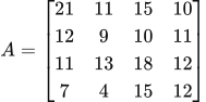 LaTeX:
A=\begin{bmatrix}21&11&15&10\\12&9&10&11\\11&13&18&12\\7&4&15&12\end{bmatrix}Top-left window
Step 1: select the four entries.
[21, 11, 12, 9]
Step 2: choose the largest entry.
 LaTeX:
y_{\max}=21Step 3: add all entries.
 LaTeX:
21+11+12+9=53Step 4: divide the sum by four for the average.
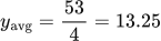 LaTeX:
y_{\mathrm{avg}}=\frac{53}4=13.25Top-right window
Step 1: select the four entries.
[15, 10, 10, 11]
Step 2: choose the largest entry.
 LaTeX:
y_{\max}=15Step 3: add all entries.
 LaTeX:
15+10+10+11=46Step 4: divide the sum by four for the average.
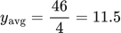 LaTeX:
y_{\mathrm{avg}}=\frac{46}4=11.5Bottom-left window
Step 1: select the four entries.
[11, 13, 7, 4]
Step 2: choose the largest entry.
 LaTeX:
y_{\max}=13Step 3: add all entries.
 LaTeX:
11+13+7+4=35Step 4: divide the sum by four for the average.
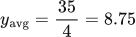 LaTeX:
y_{\mathrm{avg}}=\frac{35}4=8.75Bottom-right window
Step 1: select the four entries.
[18, 12, 15, 12]
Step 2: choose the largest entry.
 LaTeX:
y_{\max}=18Step 3: add all entries.
 LaTeX:
18+12+15+12=57Step 4: divide the sum by four for the average.
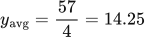 LaTeX:
y_{\mathrm{avg}}=\frac{57}4=14.25Outputs are max  LaTeX:
\begin{bmatrix}21 & 15\\13 & 18\end{bmatrix} and average 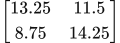 LaTeX:
\begin{bmatrix}13.25 & 11.5\\8.75 & 14.25\end{bmatrix}.
Pooling reduces spatial size and later computation and can provide limited robustness to small shifts. It can lose exact position information. It does not guarantee complete translation invariance.
Max, min and average pooling on the same lecture grid
Definition. Pooling summarizes each local window separately within each channel. Max pooling keeps its largest value, min pooling its smallest value, and average pooling its arithmetic mean. Ordinary versions have no trainable weights or biases.
Question. Apply 2 × 2 max, min and average pooling with stride 2 and no padding to the following 4 × 4 input. Give all three output matrices. (Practice: 3 marks)
Given
X = 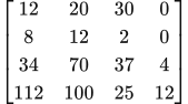 LaTeX:
\begin{bmatrix}12 & 20 & 30 & 0\\8 & 12 & 2 & 0\\34 & 70 & 37 & 4\\112 & 100 & 25 & 12\end{bmatrix}. Window = 2 × 2; stride = 2; padding = 0.
To find
The shared output shape and each of the four cells for each pooling method.
Formula — which one and why
Each output summarizes four input numbers. Use max for the largest, min for the smallest, and sum divided by 4 for the average. The window moves two cells, so these four windows do not overlap.
 LaTeX:
y_{\max}=\max(x_1,x_2,x_3,x_4)LaTeX: y_{\min}=\min(x_1,x_2,x_3,x_4) LaTeX:
y_{\mathrm{avg}}=\frac{x_1+x_2+x_3+x_4}{4}Solution — step by step
Step 1: output size. (4 −2)/2 +1 = 2. Each output has shape 2 × 2.
Step 2: top-left window [12,20,8,12]. Largest = 20; smallest = 8. Sum = 12+20+8+12 = 52. Average = 52/4 = 13.
Step 3: top-right window [30,0,2,0]. Largest = 30; smallest = 0. Sum = 30+0+2+0 = 32. Average = 32/4 = 8.
Step 4: bottom-left window [34,70,112,100]. Largest = 112; smallest = 34. Sum = 34+70+112+100 = 316. Average = 316/4 = 79.
Step 5: bottom-right window [37,4,25,12]. Largest = 37; smallest = 4. Sum = 37+4+25+12 = 78. Average = 78/4 = 19.5. Do not silently round this to 20.
Step 6: put each result back in its window's position. Max =  LaTeX:
\begin{bmatrix}20 & 30\\112 & 37\end{bmatrix}. Min =  LaTeX:
\begin{bmatrix}8 & 0\\34 & 4\end{bmatrix}. Average =  LaTeX:
\begin{bmatrix}13 & 8\\79 & 19.5\end{bmatrix}.
Final answer: Three 2 × 2 maps as above; zero trainable parameters for each pooling operation.
Why the choice matters
Max retains the largest activation in a feature window, which can still be negative if every entry is negative. Min retains the lowest response. Average retains an overall response but can dilute a sharp local peak. On raw intensity images, min can retain a dark stroke and max can retain a bright stroke. A learned CNN feature map represents filter responses; the best pooling choice is not determined solely by the original background colour.
Pooling has no parameters to update, but gradients can still pass through it. For a unique max, the upstream gradient is routed to the winning input. For an average over four inputs, each receives one-fourth of that gradient. Fewer pooled activations can reduce a later dense layer's parameter count; they do not change the size of an earlier convolution's filter.
Yaad rakho: Max = sabse bada; min = sabse chhota; average = sab jodo, count se divide.
Drill 34 Max and average pooling
Question
Question. Pool the input A shown below with 2 × 2 windows and stride 2. Find max and average outputs.
Answer — step by step
Given
Input A is printed with the question.
Window size = 2 × 2; stride = 2; no padding.
To find
Find the complete max-pooling and average-pooling outputs.
Formula — which one and why
Pooling. Max pooling selects the largest window entry. Average pooling adds its entries and divides by their count. Each channel is pooled separately.
V = current pooling window; n = number of entries in that window. Pooling learns no weights or biases.
LaTeX: y_{\max}=\max VLaTeX: y_{\mathrm{avg}}=\frac1n\sum_{v\in V}vYaad rakhne ka cue: Max mein biggest; average mein total ÷ window ka count.
Solution — step by step
Formulas and meaning
Each 2 × 2 window contains four numbers. Max pooling selects the largest of those four. Average pooling adds all four and divides by 4. Move the window by the given stride after producing one answer.
LaTeX: p_{\mathrm{max}}=\max(a_1,a_2,a_3,a_4)LaTeX: p_{\mathrm{avg}}=\frac{a_1+a_2+a_3+a_4}{4}LaTeX: N_{\mathrm{pool}}=\left\lfloor\frac{N+2P-K}{S}\right\rfloor+1Use the input size at the pooling layer. The output keeps the same channel count.
Shape: 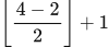 LaTeX:
\left\lfloor\frac{4-2}{2}\right\rfloor+1 = 2 on each axis; channels stay unchanged.
Pooling window (1,1)
Step 1: select the entries.
[1, 4, 0, 2]
Step 2: add all selected entries.
1 + 4 + 0 + 2 = 7
Step 3: divide by the 4 entries in this window.
7/4 = 1.75. Maximum = 4
Pooling window (1,2)
Step 1: select the entries.
[2, 3, 5, 1]
Step 2: add all selected entries.
2 + 3 + 5 + 1 = 11
Step 3: divide by the 4 entries in this window.
11/4 = 2.75. Maximum = 5
Pooling window (2,1)
Step 1: select the entries.
[6, 3, 1, 7]
Step 2: add all selected entries.
6 + 3 + 1 + 7 = 17
Step 3: divide by the 4 entries in this window.
17/4 = 4.25. Maximum = 7
Pooling window (2,2)
Step 1: select the entries.
[2, 0, 4, 8]
Step 2: add all selected entries.
2 + 0 + 4 + 8 = 14
Step 3: divide by the 4 entries in this window.
14/4 = 3.5. Maximum = 8
Average output: 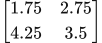 LaTeX:
\begin{bmatrix}1.75 & 2.75\\4.25 & 3.5\end{bmatrix}. Max output:  LaTeX:
\begin{bmatrix}4 & 5\\7 & 8\end{bmatrix}. Pooling normally has zero trainable parameters and reduces spatial dimensions.
Drill 40 Mixed convolution pool dense and loss
Question
Question. A is shown below, kernel Matrix 2 shown below, stride 1, valid. Apply ReLU, then 2 × 2 max pool stride 1. Flatten rowwise, use weight vector [0.1,0.2,0.3,0.4], bias 0, sigmoid output, target 1. Find all stages and BCE.
| 1 | 2 | 0 | 1 |
| 0 | 1 | 3 | 2 |
| 2 | 1 | 0 | 1 |
| 1 | 0 | 2 | 3 |
| 1 | 0 |
| 0 | −1 |
Stride 1; P = 0 (no padding).
Answer — step by step
Given
Input A and kernel Matrix 2 are printed with the question.
Conv: stride 1, valid padding; follow with ReLU.
Max pool: 2 × 2, stride 1; flatten row by row.
Dense weights = [0.1,0.2,0.3,0.4]; bias = 0; sigmoid output.
Binary target = 1.
To find
Find convolution, activated map, pooled map, flattened values, prediction and BCE.
Formula — which one and why
Convolution values. At each valid location, multiply corresponding window and kernel entries, add all products and add the filter bias once. Move by the stated stride and repeat.
X = input; K = kernel; S = stride; b = filter bias; u,v locate a kernel entry. Use the printed kernel without flipping under the stated deep-learning convention.
LaTeX: Y_{ij}=\sum_{u,v}X_{iS+u,jS+v}K_{uv}+bYaad rakhne ka cue: Matching cells multiply; sab products add; bias sirf ek baar.
Pooling. Max pooling selects the largest window entry. Average pooling adds its entries and divides by their count. Each channel is pooled separately.
V = current pooling window; n = number of entries in that window. Pooling learns no weights or biases.
LaTeX: y_{\max}=\max VLaTeX: y_{\mathrm{avg}}=\frac1n\sum_{v\in V}vYaad rakhne ka cue: Max mein biggest; average mein total ÷ window ka count.
Weighted sum and activation. Each input is multiplied by its connection weight. Add these contributions, add the bias once, then apply the stated activation.
xᵢ = input i; wᵢ = its weight; b = bias; z = sum before activation; a = output after activation; f = the specified activation function.
LaTeX: z=\sum_iw_ix_i+bLaTeX: a=f(z)Yaad rakhne ka cue: Input × weight, sabka sum, bias once, phir activation.
Sigmoid and its slope. Use sigmoid when the neuron is specified to squash its preactivation into (0,1). Once its output is known, its derivative needs only output × (1−output).
z = preactivation; p = sigmoid output; e is the exponential base, not a prediction error in this formula.
LaTeX: p=\frac{1}{1+e^{-z}}LaTeX: \frac{dp}{dz}=p(1-p)Yaad rakhne ka cue: Sigmoid output p; uska slope p × (1−p).
Binary cross-entropy. For a binary target, choose the probability of the correct outcome and take its negative natural log. Sigmoid plus BCE has combined logit derivative p−y.
y is 0 or 1; p is the predicted probability of class 1; z is the sigmoid logit. The p−y derivative already includes the sigmoid derivative.
LaTeX: L=-[y\ln p+(1-y)\ln(1-p)]LaTeX: \frac{\partial L}{\partial z}=p-yYaad rakhne ka cue: Binary target 1 ho toh −ln(p); target 0 ho toh −ln(1−p).
Solution — step by step
Formulas and the operation we are performing
A filter window produces one output value. Multiply entries at matching positions and add the products. In this deep-learning convention, keep the filter in its printed orientation.
LaTeX: Y_{ij}=\sum_{u=0}^{K_h-1}\sum_{v=0}^{K_w-1}X_{iS+u,jS+v}K_{uv}+bHere i and j identify an output position; u and v count positions inside its window. S is stride, and b is the filter bias, zero in this question. The equation uses a padded input if padding is present and zero-based indices; the working below labels output positions from 1 for readability.
LaTeX: N_{\mathrm{out}}=\left\lfloor\frac{N+2P-K}{S}\right\rfloor+1N is input width/height, P is padding per side, and K is filter width/height. Floor means take the integer below the result, then add one.
Formulas and meaning
Each 2 × 2 window contains four numbers. Max pooling selects the largest of those four. Average pooling adds all four and divides by 4. Move the window by the given stride after producing one answer.
LaTeX: p_{\mathrm{max}}=\max(a_1,a_2,a_3,a_4)LaTeX: p_{\mathrm{avg}}=\frac{a_1+a_2+a_3+a_4}{4}LaTeX: N_{\mathrm{pool}}=\left\lfloor\frac{N+2P-K}{S}\right\rfloor+1Use the input size at the pooling layer. The output keeps the same channel count.
Completing the network after pooling
Flatten row by row. Multiply the resulting entries by the dense weights and add bias. Apply sigmoid to produce p. For target 1, binary cross-entropy is minus ln(p).
LaTeX: z=\sum_iw_ix_i+b,\qquad p=\frac1{1+e^{-z}},\qquad L=-\ln pFollow each selected input window below. Matching row colors connect its input cells, kernel coefficients and products; the outlined output cell shows where their sum belongs.
Step 1 shape: LaTeX: \left\lfloor\frac{4+2 \times 0-2}{1}\right\rfloor+1 = 3 along each axis. Use the deep-learning cross-correlation convention: do not flip the printed kernel.
Output position (1, 1)
Use this position's input window. Multiply corresponding entries row by row; then add all row totals.
Input rows 1–2, columns 1–2. The window moves 1 cell per output step.
| 1 | 2 | 0 | 1 |
| 0 | 1 | 3 | 2 |
| 2 | 1 | 0 | 1 |
| 1 | 0 | 2 | 3 |
Only the outlined cells belong to this output.
| 1 | 0 |
| 0 | −1 |
Same row and column positions; no matrix multiplication.
| 1 | 0 |
| 0 | −1 |
Each cell is input × matching kernel coefficient.
1 + (−1) = 0
| 0 | −1 | −2 |
| −1 | 1 | 2 |
| 2 | −1 | −3 |
Output row 1, column 1.
Window row 1.
LaTeX: R_1=(1)\times(1)+(2)\times(0)=1Window row 2.
LaTeX: R_2=(0)\times(0)+(1)\times(-1)=-1Add the rows to obtain one output cell.
LaTeX: Y_{1,1}=(1)+(-1)=0Output position (1, 2)
Use this position's input window. Multiply corresponding entries row by row; then add all row totals.
Input rows 1–2, columns 2–3. The window moves 1 cell per output step.
| 1 | 2 | 0 | 1 |
| 0 | 1 | 3 | 2 |
| 2 | 1 | 0 | 1 |
| 1 | 0 | 2 | 3 |
Only the outlined cells belong to this output.
| 1 | 0 |
| 0 | −1 |
Same row and column positions; no matrix multiplication.
| 2 | 0 |
| 0 | −3 |
Each cell is input × matching kernel coefficient.
2 + (−3) = −1
| 0 | −1 | −2 |
| −1 | 1 | 2 |
| 2 | −1 | −3 |
Output row 1, column 2.
Window row 1.
LaTeX: R_1=(2)\times(1)+(0)\times(0)=2Window row 2.
LaTeX: R_2=(1)\times(0)+(3)\times(-1)=-3Add the rows to obtain one output cell.
LaTeX: Y_{1,2}=(2)+(-3)=-1Output position (1, 3)
Use this position's input window. Multiply corresponding entries row by row; then add all row totals.
Input rows 1–2, columns 3–4. The window moves 1 cell per output step.
| 1 | 2 | 0 | 1 |
| 0 | 1 | 3 | 2 |
| 2 | 1 | 0 | 1 |
| 1 | 0 | 2 | 3 |
Only the outlined cells belong to this output.
| 1 | 0 |
| 0 | −1 |
Same row and column positions; no matrix multiplication.
| 0 | 0 |
| 0 | −2 |
Each cell is input × matching kernel coefficient.
0 + (−2) = −2
| 0 | −1 | −2 |
| −1 | 1 | 2 |
| 2 | −1 | −3 |
Output row 1, column 3.
Window row 1.
LaTeX: R_1=(0)\times(1)+(1)\times(0)=0Window row 2.
LaTeX: R_2=(3)\times(0)+(2)\times(-1)=-2Add the rows to obtain one output cell.
LaTeX: Y_{1,3}=(0)+(-2)=-2Output position (2, 1)
Use this position's input window. Multiply corresponding entries row by row; then add all row totals.
Input rows 2–3, columns 1–2. The window moves 1 cell per output step.
| 1 | 2 | 0 | 1 |
| 0 | 1 | 3 | 2 |
| 2 | 1 | 0 | 1 |
| 1 | 0 | 2 | 3 |
Only the outlined cells belong to this output.
| 1 | 0 |
| 0 | −1 |
Same row and column positions; no matrix multiplication.
| 0 | 0 |
| 0 | −1 |
Each cell is input × matching kernel coefficient.
0 + (−1) = −1
| 0 | −1 | −2 |
| −1 | 1 | 2 |
| 2 | −1 | −3 |
Output row 2, column 1.
Window row 1.
LaTeX: R_1=(0)\times(1)+(1)\times(0)=0Window row 2.
LaTeX: R_2=(2)\times(0)+(1)\times(-1)=-1Add the rows to obtain one output cell.
LaTeX: Y_{2,1}=(0)+(-1)=-1Output position (2, 2)
Use this position's input window. Multiply corresponding entries row by row; then add all row totals.
Input rows 2–3, columns 2–3. The window moves 1 cell per output step.
| 1 | 2 | 0 | 1 |
| 0 | 1 | 3 | 2 |
| 2 | 1 | 0 | 1 |
| 1 | 0 | 2 | 3 |
Only the outlined cells belong to this output.
| 1 | 0 |
| 0 | −1 |
Same row and column positions; no matrix multiplication.
| 1 | 0 |
| 0 | 0 |
Each cell is input × matching kernel coefficient.
1 + 0 = 1
| 0 | −1 | −2 |
| −1 | 1 | 2 |
| 2 | −1 | −3 |
Output row 2, column 2.
Window row 1.
LaTeX: R_1=(1)\times(1)+(3)\times(0)=1Window row 2.
LaTeX: R_2=(1)\times(0)+(0)\times(-1)=0Add the rows to obtain one output cell.
LaTeX: Y_{2,2}=(1)+(0)=1Output position (2, 3)
Use this position's input window. Multiply corresponding entries row by row; then add all row totals.
Input rows 2–3, columns 3–4. The window moves 1 cell per output step.
| 1 | 2 | 0 | 1 |
| 0 | 1 | 3 | 2 |
| 2 | 1 | 0 | 1 |
| 1 | 0 | 2 | 3 |
Only the outlined cells belong to this output.
| 1 | 0 |
| 0 | −1 |
Same row and column positions; no matrix multiplication.
| 3 | 0 |
| 0 | −1 |
Each cell is input × matching kernel coefficient.
3 + (−1) = 2
| 0 | −1 | −2 |
| −1 | 1 | 2 |
| 2 | −1 | −3 |
Output row 2, column 3.
Window row 1.
LaTeX: R_1=(3)\times(1)+(2)\times(0)=3Window row 2.
LaTeX: R_2=(0)\times(0)+(1)\times(-1)=-1Add the rows to obtain one output cell.
LaTeX: Y_{2,3}=(3)+(-1)=2Output position (3, 1)
Use this position's input window. Multiply corresponding entries row by row; then add all row totals.
Input rows 3–4, columns 1–2. The window moves 1 cell per output step.
| 1 | 2 | 0 | 1 |
| 0 | 1 | 3 | 2 |
| 2 | 1 | 0 | 1 |
| 1 | 0 | 2 | 3 |
Only the outlined cells belong to this output.
| 1 | 0 |
| 0 | −1 |
Same row and column positions; no matrix multiplication.
| 2 | 0 |
| 0 | 0 |
Each cell is input × matching kernel coefficient.
2 + 0 = 2
| 0 | −1 | −2 |
| −1 | 1 | 2 |
| 2 | −1 | −3 |
Output row 3, column 1.
Window row 1.
LaTeX: R_1=(2)\times(1)+(1)\times(0)=2Window row 2.
LaTeX: R_2=(1)\times(0)+(0)\times(-1)=0Add the rows to obtain one output cell.
LaTeX: Y_{3,1}=(2)+(0)=2Output position (3, 2)
Use this position's input window. Multiply corresponding entries row by row; then add all row totals.
Input rows 3–4, columns 2–3. The window moves 1 cell per output step.
| 1 | 2 | 0 | 1 |
| 0 | 1 | 3 | 2 |
| 2 | 1 | 0 | 1 |
| 1 | 0 | 2 | 3 |
Only the outlined cells belong to this output.
| 1 | 0 |
| 0 | −1 |
Same row and column positions; no matrix multiplication.
| 1 | 0 |
| 0 | −2 |
Each cell is input × matching kernel coefficient.
1 + (−2) = −1
| 0 | −1 | −2 |
| −1 | 1 | 2 |
| 2 | −1 | −3 |
Output row 3, column 2.
Window row 1.
LaTeX: R_1=(1)\times(1)+(0)\times(0)=1Window row 2.
LaTeX: R_2=(0)\times(0)+(2)\times(-1)=-2Add the rows to obtain one output cell.
LaTeX: Y_{3,2}=(1)+(-2)=-1Output position (3, 3)
Use this position's input window. Multiply corresponding entries row by row; then add all row totals.
Input rows 3–4, columns 3–4. The window moves 1 cell per output step.
| 1 | 2 | 0 | 1 |
| 0 | 1 | 3 | 2 |
| 2 | 1 | 0 | 1 |
| 1 | 0 | 2 | 3 |
Only the outlined cells belong to this output.
| 1 | 0 |
| 0 | −1 |
Same row and column positions; no matrix multiplication.
| 0 | 0 |
| 0 | −3 |
Each cell is input × matching kernel coefficient.
0 + (−3) = −3
| 0 | −1 | −2 |
| −1 | 1 | 2 |
| 2 | −1 | −3 |
Output row 3, column 3.
Window row 1.
LaTeX: R_1=(0)\times(1)+(1)\times(0)=0Window row 2.
LaTeX: R_2=(2)\times(0)+(3)\times(-1)=-3Add the rows to obtain one output cell.
LaTeX: Y_{3,3}=(0)+(-3)=-3Final output: LaTeX: \begin{bmatrix}0 & -1 & -2\\-1 & 1 & 2\\2 & -1 & -3\end{bmatrix}. Each output came from its own complete window; stride changes the next window position, not the multiplication rule.
ReLU turns negative entries into 0: LaTeX: \begin{bmatrix}0 & 0 & 0\\0 & 1 & 2\\2 & 0 & 0\end{bmatrix}.
Shape: LaTeX: \left\lfloor\frac{3-2}{1}\right\rfloor+1 = 2 on each axis; channels stay unchanged.
Pooling window (1,1)
Step 1: select the entries.
[0, 0, 0, 1]
Step 2: add all selected entries.
0 + 0 + 0 + 1 = 1
Step 3: divide by the 4 entries in this window.
1/4 = 0.25. Maximum = 1
Pooling window (1,2)
Step 1: select the entries.
[0, 0, 1, 2]
Step 2: add all selected entries.
0 + 0 + 1 + 2 = 3
Step 3: divide by the 4 entries in this window.
3/4 = 0.75. Maximum = 2
Pooling window (2,1)
Step 1: select the entries.
[0, 1, 2, 0]
Step 2: add all selected entries.
0 + 1 + 2 + 0 = 3
Step 3: divide by the 4 entries in this window.
3/4 = 0.75. Maximum = 2
Pooling window (2,2)
Step 1: select the entries.
[1, 2, 0, 0]
Step 2: add all selected entries.
1 + 2 + 0 + 0 = 3
Step 3: divide by the 4 entries in this window.
3/4 = 0.75. Maximum = 2
Average output: LaTeX: \begin{bmatrix}0.25 & 0.75\\0.75 & 0.75\end{bmatrix}. Max output: LaTeX: \begin{bmatrix}1 & 2\\2 & 2\end{bmatrix}. Pooling normally has zero trainable parameters and reduces spatial dimensions.
Use MAX output and flatten rowwise: [1, 2, 2, 2]. Dense z = 0.1 × 1 + 0.2 × 2 + 0.3 × 2 + 0.4 × 2 = 1.9. p = σ(1.9) = 0.869891526. BCE = −ln(p) = 0.139386758. Average pool values were computed for contrast; the question requires max pool.
Convolution parameter count
A filter has one learned weight for each spatial position in each input channel. Count the weights in one filter, add its one bias, then multiply by the number of filters. Sliding a filter to many positions reuses these weights; it does not create new parameters.
LaTeX: P_{conv}=(K_hK_wC_{in}+1)C_{out}Output size and parameter count are different
Definition. Output shape specifies the size of a layer's computed tensor. Parameter count specifies the number of independent trainable coefficients. Spatial weight sharing allows a convolutional layer to produce many activations from comparatively few parameters.
Explanation and working
Question. A 7 × 7 × 3 input passes through two 3 × 3 filters, stride 2 and padding 1. Find output shape and parameter count, including bias.
Given
Input = 7 × 7 × 3; two 3 × 3 filters.
Stride = 2; padding = 1; include biases.
To find
Find the output shape and trainable parameter count.
Formula — which one and why
Convolution/pooling spatial size. Padding adds P positions at both ends. Subtract kernel width to find the last valid start, divide by stride, take the floor and include the initial placement with +1.
N = current height or width; K = kernel/window size; S = stride; P = padding per side. Apply separately to height and width; dilation is 1 here.
LaTeX: N_{\mathrm{out}}=\left\lfloor\frac{N+2P-K}{S}\right\rfloor+1Yaad rakhne ka cue: Input + dono sides ki padding − kernel; stride se divide; floor + 1.
Convolution parameters. Every filter spans all input channels. Count its spatial coefficients across those channels, add one bias and multiply by the number of filters.
K_h,K_w = filter height/width; C_in = input channels; C_out = number of filters and output channels. Spatial output positions reuse these weights.
LaTeX: N_w=K_hK_wC_{\mathrm{in}}C_{\mathrm{out}}LaTeX: N_b=C_{\mathrm{out}}LaTeX: P=N_w+N_bYaad rakhne ka cue: Filter area × input channels × filters; phir ek bias per filter.
Solution — step by step
Step 1 spatial size: padding adds two, giving 7 + 2 − 3 = 6. Divide by stride: 6 ÷ 2 = 3. Apply floor and add the first position: 3 + 1 = 4. There are two filters, so output is 4 × 4 × 2.
Step 2 parameters: one filter has 3 × 3 × 3 = 27 weights and one bias, giving 28. Two filters have 56 parameters. The 4 × 4 output positions reuse those weights; they do not create 16 new sets of parameters.
Model answer: shape, activations and parameters
Question
Question. Distinguish a CNN layer's output shape, number of output activations and number of trainable parameters. Explain the formulas used to calculate them.
Answer — step by step
Output shape tells how the produced values are arranged. The activation count tells how many values were produced for one input. Parameter count tells how many learned weights and biases define the layer. These are three different questions.
Spatial output shape
For an ordinary convolution with dilation 1:
LaTeX: N_{\mathrm{out}}=\left\lfloor\frac{N+2P-K}{S}\right\rfloor+1N is the incoming spatial size, P is padding on each side, K is kernel size and S is stride. Apply the rule independently to height and width. The number of output channels is the number of filters.
Output activations
 LaTeX:
A=H_{\mathrm{out}}W_{\mathrm{out}}C_{\mathrm{out}}This is the number of output values for one example, excluding any batch dimension.
Trainable parameters
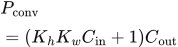 LaTeX:
P_{\mathrm{conv}}=(K_hK_wC_{\mathrm{in}}+1)C_{\mathrm{out}}Each filter spans every incoming channel. The +1 is one bias per filter. Remove it if biases are disabled. Spatial output dimensions do not appear here because filters share their weights across positions.
Small example
A 7 × 7 × 3 input, two 3 × 3 filters, stride 2 and padding 1 gives output 4 × 4 × 2. It contains 32 activations but has (3 × 3 × 3 + 1) × 2 = 56 parameters. These counts do not need to match. In a multilayer question, the current layer's output channels become the next convolution's input channels.
Faculty CNN table: shapes, activations and 62958 parameters
Question. A CNN receives a 32 × 32 × 3 image. It uses Conv1: eight 5 × 5 filters, stride 1, no padding; Pool1: 2 × 2, stride 2; Conv2: sixteen 5 × 5 filters, stride 1, no padding; Pool2: 2 × 2, stride 2; flatten; dense 120; dense 84; dense 10 followed by softmax. Include one bias per filter or receiving dense neuron. Find every output shape, activation count and trainable-parameter count. (Practice: 10 marks)
Given
Input = 32 × 32 × 3. Both convolutions are ordinary full-channel convolutions. Pooling has no padding. Dense widths are 120, 84 and 10. No batch-normalization layer is present in this particular question.
To find
Output shape and number of output values for each layer, its trainable parameters, and the total parameters.
Formula — which one and why
Use the spatial-size formula for each convolution/pool. Use one full-depth kernel plus one bias per convolutional filter. Flattening counts all remaining values before the first dense layer. Each dense neuron then receives one weight per input plus one bias.
LaTeX: N_{\mathrm{out}}=\left\lfloor\frac{N+2P-K}{S}\right\rfloor+1LaTeX: A=H_{\mathrm{out}}W_{\mathrm{out}}C_{\mathrm{out}}LaTeX: P_{\mathrm{conv}}=(K_hK_wC_{\mathrm{in}}+1)C_{\mathrm{out}} LaTeX:
P_{\mathrm{dense}}=(n_{\mathrm{in}}+1)n_{\mathrm{out}}A counts produced activations. P_conv and P_dense count independent learned coefficients. They are not the same quantity. Pooling, flattening and softmax itself add zero learned parameters here.
Solution — step by step
Step 1: input. Shape = 32 × 32 × 3. Values = 32×32×3 = 3,072. Trainable parameters = 0.
Step 2: Conv1 spatial size. (32−5)/1 +1 = 28. Eight filters give shape 28 × 28 × 8. Activations = 28×28×8 = 6,272.
Step 3: Conv1 parameters. One filter contains 5×5×3 = 75 weights. Add one bias: 76. Multiply by eight filters: 76×8 = 608.
Step 4: Pool1. (28−2)/2 +1 = 14. Shape = 14 × 14 × 8. Activations = 14×14×8 = 1,568. Parameters = 0; channel count remains eight.
Step 5: Conv2 spatial size. (14−5)/1 +1 = 10. Sixteen filters give shape 10 × 10 × 16. Activations = 1,600.
Step 6: Conv2 parameters. Its input has eight channels. Each filter has 5×5×8 = 200 weights, then one bias. Total = 201×16 = 3,216.
Step 7: Pool2 and flatten. (10−2)/2 +1 = 5. Pool shape = 5 × 5 × 16. Flattened length = 5×5×16 = 400. Neither operation adds parameters.
Step 8: dense 120. Weights = 400×120 = 48,000. Biases = 120. Parameters = 48,120. Output contains 120 activations.
Step 9: dense 84. Weights = 120×84 = 10,080. Biases = 84. Parameters = 10,164. Output contains 84 activations.
Step 10: dense 10 and softmax. Weights = 84×10 = 840. Biases = 10. Dense parameters = 850. Softmax converts the ten logits into ten probabilities and adds zero parameters. A table naming the combined classifier row “Softmax” attributes these 850 parameters to its preceding dense transformation.
Step 11: add only the trainable counts. 608+3,216 = 3,824; +48,120 = 51,944; +10,164 = 62,108; +850 = 62,958.
| Layer | Output shape | Activations | Parameters |
|---|---|---|---|
| Input | 32 × 32 × 3 | 3,072 | 0 |
| Conv1 | 28 × 28 × 8 | 6,272 | 608 |
| Pool1 | 14 × 14 × 8 | 1,568 | 0 |
| Conv2 | 10 × 10 × 16 | 1,600 | 3,216 |
| Pool2 / flatten | 5 × 5 × 16 / 400 | 400 | 0 |
| Dense 120 | 120 | 120 | 48,120 |
| Dense 84 | 84 | 84 | 10,164 |
| Dense 10 → softmax | 10 | 10 | 850 + 0 |
Final answer: The network has 62,958 trainable parameters. This is the specified classroom CNN, not a universal parameter total for every LeNet-like network.
Yaad rakho: Shape aage carry karo; weights aur activations ko alag columns mein rakho.
Parameters are different from activation values
Definition. Parameters are learned coefficients shared across evaluations. Activations are input-dependent values computed during a forward pass. The number of activation values therefore differs from the number of trainable parameters.
Explanation and working
An activation is a number produced for a particular input. A parameter is a learned number reused across inputs. A 100 × 100 feature map can be produced by a filter with only a few weights.
LaTeX: P_{\mathrm{conv}}=(K_hK_wC_{\mathrm{in}}+1)C_{\mathrm{out}}The +1 is one bias per filter. If bias is explicitly disabled, remove it. Height and width of the image do not enter the parameter formula; they enter the number of output activations and the amount of computation.
One filter, then all filters
Question. A 3 × 3 convolution receives 3 input channels and has 16 filters, each with one bias. Find its trainable parameters and output-channel count.
Given
Kernel = 3 × 3; input channels = 3; filters = 16; one bias per filter.
To find
Weights, biases, total trainable parameters and output channels.
Formula — which one and why
Each filter spans every input channel and owns one bias. Spatial reuse does not create extra weights.
Kₕ,Kw are kernel dimensions; Cᵢₙ is input depth; Cₒᵤₜ is the number of filters.
 LaTeX:
P=(K_hK_wC_{\mathrm{in}}+1)C_{\mathrm{out}}Yaad rakhne ka cue: Ek filter ka count banao, phir filters se multiply.
Solution — step by step
Step 1: count weights in one filter.
 LaTeX:
3(3)(3)=27Step 2: include its one bias.
 LaTeX:
27+1=28Step 3: count all weights.
 LaTeX:
27(16)=432Step 4: count all biases.
 LaTeX:
1(16)=16Step 5: add and state channel count.
 LaTeX:
P=432+16=448Each filter produces one channel, so output channels = 16.
Final answer: 432 weights + 16 biases = 448 trainable parameters; 16 output channels.
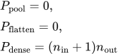 LaTeX:
P_{\mathrm{pool}}=0,\quad P_{\mathrm{flatten}}=0,\quad P_{\mathrm{dense}}=(n_{\mathrm{in}}+1)n_{\mathrm{out}}Flatten rearranges H × W × C activation values into one vector of length HWC. It does not learn anything. A following dense layer connects to every one of those values.
Drill 35 Complete small CNN
Question
Question. Input 10 × 10 × 1 → Conv 3 × 3,4 filters, stride 1, valid → Pool 2 stride 2 → Flatten → Dense 3. Find all shapes and parameters.
Answer — step by step
Given
Input = 10 × 10 × 1.
Conv: 3 × 3, 4 filters, stride 1, valid padding.
Pool: 2 × 2, stride 2; then flatten and dense layer with 3 outputs.
Include one bias per filter/dense neuron.
To find
Find all output shapes, layer parameter counts and their sum.
Formula — which one and why
Complete CNN calculation. Carry each output shape into the next layer. Convolution changes spatial size and channel count; pooling changes spatial size; flattening converts all activations into dense-layer inputs.
H,W,C = feature-map height, width and channels; K = kernel size; S = stride; P_pad = padding. One bias is assumed for each learned filter or dense neuron unless specified otherwise.
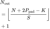 LaTeX:
N_{\mathrm{out}}=\left\lfloor\frac{N+2P_{\mathrm{pad}}-K}{S}\right\rfloor+1 LaTeX:
P_{\mathrm{conv}}=(K^2C_{\mathrm{in}}+1)C_{\mathrm{out}} LaTeX:
n_{\mathrm{flat}}=HWCLaTeX: P_{\mathrm{dense}}=(n_{\mathrm{in}}+1)n_{\mathrm{out}} LaTeX:
P_{\mathrm{pool}}=P_{\mathrm{flatten}}=0Yaad rakhne ka cue: Ek layer ka output, next layer ka input; shape aur parameters alag count.
Solution — step by step
Formulas and assumptions
“Valid” means zero padding. The convolution and dense layers each have one bias per receiving filter or neuron. Pooling and flattening have no learned parameters.
LaTeX: N_{\mathrm{out}}=\left\lfloor\frac{N+2P-K}{S}\right\rfloor+1LaTeX: P_{\mathrm{conv}}=(K^2C_{\mathrm{in}}+1)C_{\mathrm{out}}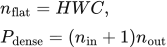 LaTeX:
n_{\mathrm{flat}}=HWC,\qquad P_{\mathrm{dense}}=(n_{\mathrm{in}}+1)n_{\mathrm{out}}Step 1: convolution shape
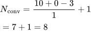 LaTeX:
N_{\mathrm{conv}}=\frac{10+0-3}{1}+1=7+1=8Four filters produce four channels: 8 × 8 × 4.
Step 2: convolution parameters
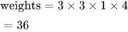 LaTeX:
\text{weights}=3\times3\times1\times4=36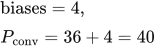 LaTeX:
\text{biases}=4,\qquad P_{\mathrm{conv}}=36+4=40Step 3: pooling shape
Pooling now receives size 8, not the original size 10.
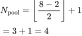 LaTeX:
N_{\mathrm{pool}}=\left\lfloor\frac{8-2}{2}\right\rfloor+1=3+1=4Channels remain 4: 4 × 4 × 4. Pooling parameters = 0.
Step 4: flatten
 LaTeX:
n_{\mathrm{flat}}=4\times4\times4=64Flatten creates a vector of 64 numbers. It rearranges values, so its parameter count is 0.
Step 5: dense layer with 3 outputs
 LaTeX:
\text{weights}=64\times3=192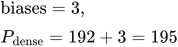 LaTeX:
\text{biases}=3,\qquad P_{\mathrm{dense}}=192+3=195Step 6: add learned parameters
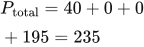 LaTeX:
P_{\mathrm{total}}=40+0+0+195=235Final answer: shapes 8 × 8 × 4 → 4 × 4 × 4 → 64 → 3; total 235 parameters.
Flatten and dense parameter count
Flattening rearranges all activation values into a list. It learns no new numbers. A dense layer then connects every value in that list to every receiving neuron; each receiving neuron also has one bias.
 LaTeX:
N_{flat}=HWC LaTeX:
P_{dense}=(N_{in}+1)N_{out}Counting parameters in a dense network
Definition. A dense layer connects every input component to every receiving neuron. Its trainable parameters are these connection weights and the receiving neurons' independently trainable biases.
Deriving the parameter count
For m inputs and n receiving neurons, each receiver needs m weights. There are therefore mn weights. With one bias per receiver, there are n additional parameters:
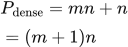 LaTeX:
P_{\mathrm{dense}}=mn+n=(m+1)nActivation values are computed from data and parameters; they are not additional trainable parameters. The input layer supplies data and does not acquire an extra bias merely because it appears in a diagram.
Complete numerical
Question. A network has 10 input features, three hidden layers with 5 neurons each, and 4 outputs. Every receiving neuron has a bias. Count its trainable parameters.
Given
Layer sizes: 10 inputs → 5 hidden → 5 hidden → 5 hidden → 4 outputs.
Every hidden/output neuron has one bias.
To find
Count weights and biases at each receiving layer, then the total.
Formula — which one and why
Dense-layer parameters. Every output neuron receives every input, so multiply inputs by outputs for weights. Add one bias per receiving neuron. Sum separate layers.
n_in = incoming features; n_out = receiving neurons. The input layer itself has no learned receiving weights or biases.
 LaTeX:
P=(n_{\mathrm{in}}+1)n_{\mathrm{out}}Yaad rakhne ka cue: Har output ke liye saare inputs plus ek bias.
Solution — step by step
Step 1: identify the consecutive layer widths.
 LaTeX:
10\longrightarrow5\longrightarrow5\longrightarrow5\longrightarrow4There are four trainable dense transformations. A connection between two hidden layers is counted once, as part of the receiving layer's parameters.
Step 2: count weights and biases for each transformation.
| Transformation | Weights | Biases | Layer total |
|---|---|---|---|
| Input → hidden 1 | 10 × 5 = 50 | 5 | 55 |
| Hidden 1 → hidden 2 | 5 × 5 = 25 | 5 | 30 |
| Hidden 2 → hidden 3 | 5 × 5 = 25 | 5 | 30 |
| Hidden 3 → output | 5 × 4 = 20 | 4 | 24 |
Step 3: add the layer totals.
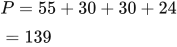 LaTeX:
P=55+30+30+24=139Equivalently, the network has 120 weights and 19 biases, so 120 + 19 = 139.
Final answer: 139 trainable parameters. If a question explicitly removes biases, count only the 120 weights. Optimizer states such as Adam's moments are extra training storage, not extra parameters in this predictive network.
One complete CNN pipeline
Question. Input 128 × 128 × 3 → convolution 3 × 3, 16 filters, stride 1, no padding → pooling 2 × 2, stride 2 → convolution 3 × 3, 32 filters, stride 1, no padding → pooling 2 × 2, stride 2 → dense 240 → dense 120 → dense 5 with softmax. Find every output shape and trainable parameter count. Assume one bias per receiving filter or dense neuron.
Given
Input = 128 × 128 × 3.
Conv: 3 × 3,16 filters,stride 1,valid → pool 2,stride 2.
Conv: 3 × 3,32 filters,stride 1,valid → pool 2,stride 2.
Flatten → dense 240 → dense 120 → dense 5.
One bias per learned filter/dense neuron.
To find
Find every output shape and layer parameter count, then the network total.
Formula — which one and why
Complete CNN calculation. Carry each output shape into the next layer. Convolution changes spatial size and channel count; pooling changes spatial size; flattening converts all activations into dense-layer inputs.
H,W,C = feature-map height, width and channels; K = kernel size; S = stride; P_pad = padding. One bias is assumed for each learned filter or dense neuron unless specified otherwise.
LaTeX: N_{\mathrm{out}}=\left\lfloor\frac{N+2P_{\mathrm{pad}}-K}{S}\right\rfloor+1LaTeX: P_{\mathrm{conv}}=(K^2C_{\mathrm{in}}+1)C_{\mathrm{out}}LaTeX: n_{\mathrm{flat}}=HWCLaTeX: P_{\mathrm{dense}}=(n_{\mathrm{in}}+1)n_{\mathrm{out}}LaTeX: P_{\mathrm{pool}}=P_{\mathrm{flatten}}=0Yaad rakhne ka cue: Ek layer ka output, next layer ka input; shape aur parameters alag count.
Solution — step by step
Step 1. Conv 1 size. (128 − 3)/1 + 1 = 126; output 126 × 126 × 16. Parameters = (3 × 3 × 3 + 1) × 16 = 448.
Step 2. Pool 1 size. 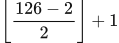 LaTeX:
\left\lfloor\frac{126 - 2}{2}\right\rfloor+1 = 63; output 63 × 63 × 16. Parameters = 0.
Step 3. Conv 2 size. (63 − 3)/1 + 1 = 61; output 61 × 61 × 32. Input channels are now 16, not the original 3. Parameters = (3 × 3 × 16 + 1) × 32 = 4,640.
Step 4. Pool 2 size. 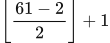 LaTeX:
\left\lfloor\frac{61 - 2}{2}\right\rfloor+1 =  LaTeX:
\left\lfloor 29.5\right\rfloor + 1 = 30; output 30 × 30 × 32. Parameters = 0.
Step 5. Flatten. 30 × 30 × 32 = 28,800 values. Parameters = 0.
Step 6. Dense 240. 28,800 weights per neuron plus one bias, multiplied by 240: (28,800 + 1) × 240 = 6,912,240.
Step 7. Dense 120. (240 + 1) × 120 = 28,920.
Step 8. Classifier. (120 + 1) × 5 = 605. Softmax itself adds no extra parameters; these 605 belong to the dense class-score layer.
Step 9. Total. 448 + 4,640 + 6,912,240 + 28,920 + 605 = 6,946,853. Most parameters come from the first dense layer.
Drill 35 Complete small CNN
Question
Question. Input 10 × 10 × 1 → Conv 3 × 3,4 filters, stride 1, valid → Pool 2 stride 2 → Flatten → Dense 3. Find all shapes and parameters.
Answer — step by step
Given
Input = 10 × 10 × 1.
Conv: 3 × 3, 4 filters, stride 1, valid padding.
Pool: 2 × 2, stride 2; then flatten and dense layer with 3 outputs.
Include one bias per filter/dense neuron.
To find
Find all output shapes, layer parameter counts and their sum.
Formula — which one and why
Complete CNN calculation. Carry each output shape into the next layer. Convolution changes spatial size and channel count; pooling changes spatial size; flattening converts all activations into dense-layer inputs.
H,W,C = feature-map height, width and channels; K = kernel size; S = stride; P_pad = padding. One bias is assumed for each learned filter or dense neuron unless specified otherwise.
LaTeX: N_{\mathrm{out}}=\left\lfloor\frac{N+2P_{\mathrm{pad}}-K}{S}\right\rfloor+1LaTeX: P_{\mathrm{conv}}=(K^2C_{\mathrm{in}}+1)C_{\mathrm{out}}LaTeX: n_{\mathrm{flat}}=HWCLaTeX: P_{\mathrm{dense}}=(n_{\mathrm{in}}+1)n_{\mathrm{out}}LaTeX: P_{\mathrm{pool}}=P_{\mathrm{flatten}}=0Yaad rakhne ka cue: Ek layer ka output, next layer ka input; shape aur parameters alag count.
Solution — step by step
Formulas and assumptions
“Valid” means zero padding. The convolution and dense layers each have one bias per receiving filter or neuron. Pooling and flattening have no learned parameters.
LaTeX: N_{\mathrm{out}}=\left\lfloor\frac{N+2P-K}{S}\right\rfloor+1LaTeX: P_{\mathrm{conv}}=(K^2C_{\mathrm{in}}+1)C_{\mathrm{out}}LaTeX: n_{\mathrm{flat}}=HWC,\qquad P_{\mathrm{dense}}=(n_{\mathrm{in}}+1)n_{\mathrm{out}}Step 1: convolution shape
LaTeX: N_{\mathrm{conv}}=\frac{10+0-3}{1}+1=7+1=8Four filters produce four channels: 8 × 8 × 4.
Step 2: convolution parameters
LaTeX: \text{weights}=3\times3\times1\times4=36LaTeX: \text{biases}=4,\qquad P_{\mathrm{conv}}=36+4=40Step 3: pooling shape
Pooling now receives size 8, not the original size 10.
LaTeX: N_{\mathrm{pool}}=\left\lfloor\frac{8-2}{2}\right\rfloor+1=3+1=4Channels remain 4: 4 × 4 × 4. Pooling parameters = 0.
Step 4: flatten
LaTeX: n_{\mathrm{flat}}=4\times4\times4=64Flatten creates a vector of 64 numbers. It rearranges values, so its parameter count is 0.
Step 5: dense layer with 3 outputs
LaTeX: \text{weights}=64\times3=192LaTeX: \text{biases}=3,\qquad P_{\mathrm{dense}}=192+3=195Step 6: add learned parameters
LaTeX: P_{\mathrm{total}}=40+0+0+195=235Final answer: shapes 8 × 8 × 4 → 4 × 4 × 4 → 64 → 3; total 235 parameters.
Drill 43 Mixed CNN dimensions softmax and loss
Question
Question. Input 8 × 8 × 3 → Conv 3, stride 1, padding 1, 2 filters → Pool 2, stride 2 → Flatten → Dense 3. Logits [0,1,−1], true class is the second class (one-hot target [0,1,0]). Find shapes, parameters, probabilities and CCE.
Answer — step by step
Given
Input = 8 × 8 × 3.
Conv: kernel 3, stride 1, padding 1, 2 filters.
Pool: kernel 2, stride 2; flatten; dense layer with 3 outputs.
Logits = [0,1,−1]; true class is the second class (one-hot target [0,1,0]).
To find
Find shapes, parameter counts, probabilities and CCE.
Formula — which one and why
Complete CNN calculation. Carry each output shape into the next layer. Convolution changes spatial size and channel count; pooling changes spatial size; flattening converts all activations into dense-layer inputs.
H,W,C = feature-map height, width and channels; K = kernel size; S = stride; P_pad = padding. One bias is assumed for each learned filter or dense neuron unless specified otherwise.
LaTeX: N_{\mathrm{out}}=\left\lfloor\frac{N+2P_{\mathrm{pad}}-K}{S}\right\rfloor+1LaTeX: P_{\mathrm{conv}}=(K^2C_{\mathrm{in}}+1)C_{\mathrm{out}}LaTeX: n_{\mathrm{flat}}=HWCLaTeX: P_{\mathrm{dense}}=(n_{\mathrm{in}}+1)n_{\mathrm{out}}LaTeX: P_{\mathrm{pool}}=P_{\mathrm{flatten}}=0Yaad rakhne ka cue: Ek layer ka output, next layer ka input; shape aur parameters alag count.
Stable softmax. Exponentiate each logit and divide by the sum. Subtracting the largest logit first keeps the exponentials numerically manageable and leaves the probabilities unchanged.
zⱼ = class j score; M = largest score; pⱼ = class j probability. All probabilities sum to 1.
LaTeX: M=\max_j z_jLaTeX: p_j=\frac{e^{z_j-M}}{\sum_k e^{z_k-M}}Yaad rakhne ka cue: Largest score ghatao, exp nikalo, total se sabko divide karo.
Categorical cross-entropy. For mutually exclusive classes with a one-hot target, all zero-target terms disappear. The loss is the negative log of the probability assigned to the true class.
yⱼ = target entry; pⱼ = predicted probability; c = index of the true class. Use natural logarithms unless another base is specified.
LaTeX: L=-\sum_j y_j\ln p_jLaTeX: L=-\ln p_cYaad rakhne ka cue: One-hot mein sirf correct class ki probability ka minus ln.
Solution — step by step
Formulas used
Separate shape from learned parameter count. H, W and C mean height, width and channels. K, P and S mean filter size, padding per side and stride.
LaTeX: N_{\mathrm{out}}=\left\lfloor\frac{N+2P-K}{S}\right\rfloor+1LaTeX: P_{\mathrm{conv}}=(K^2C_{\mathrm{in}}+1)C_{\mathrm{out}}LaTeX: n_{\mathrm{flat}}=HWC,\qquad P_{\mathrm{dense}}=(n_{\mathrm{in}}+1)n_{\mathrm{out}}The +1 counts one bias per receiving filter or neuron. Pooling and flattening add no learned parameters. Softmax converts scores to probabilities; CCE uses the probability of the correct class.
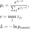 LaTeX:
p_i=\frac{e^{z_i-c}}{\sum_j e^{z_j-c}},\quad c=\max_jz_j,\quad L=-\ln p_{\mathrm{correct}}Conv size = (8+2−3)+1 = 8; output 8 × 8 × 2; parameters = (3 × 3 × 3+1) × 2 = 56. Pool 4 × 4 × 2; parameters 0. Flatten 32. Dense 3 parameters = (32+1) × 3 = 99. Total = 155.
Step 1 stabilize: subtract the largest logit 1 from every value: [-1, 0, -2]. This does not change softmax.
Step 2 exponentiate: exp values = [0.367879441, 1, 0.135335283].
Step 3 denominator: sum = 1.503214724.
Step 4 divide each value by this same sum: probabilities = [0.244728471, 0.665240956, 0.090030573]. Check: all are positive and their sum is 1 (apart from rounding); the largest logit gets the largest probability.
Correct class probability = 0.665240956; CCE = −ln(0.665240956) = 0.407605964.
Convolution multiply-accumulate count
A parameter count counts learned numbers. A multiply-accumulate count counts how many times input–weight products are used. One filter is reused at every output position, so computation includes output height and width even though its parameter count does not.
LaTeX: MAC=H_{out}W_{out}K_hK_wC_{in}C_{out}Why one by one convolution saves work
Definition. A 1 × 1 convolution combines the input channels independently at each spatial location. A bottleneck uses fewer output channels before a larger spatial convolution, reducing its parameter and multiplication counts.
Question. Input is 28 × 28 × 192. Compare a direct same-padded 5 × 5 convolution with 32 filters against a 1 × 1 reduction to 16 channels followed by the same 5 × 5 convolution. Count MACs and ignore bias additions.
Given
Both paths produce 28 × 28 × 32. The direct layer receives 192 channels; the bottleneck's spatial layer receives 16 channels. Stride is 1 and padding preserves spatial size.
To find
Direct MACs, total two-stage bottleneck MACs and percentage saved.
Formula — which one and why
Each output scalar uses one product per input-channel kernel entry. Multiply that cost by the number of output positions and channels. The two bottleneck layers require separate counts, which are added.
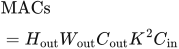 LaTeX:
\mathrm{MACs}=H_{\mathrm{out}}W_{\mathrm{out}}C_{\mathrm{out}}K^2C_{\mathrm{in}}One MAC counts one multiply–accumulate pair. A convention counting multiplication and addition separately gives approximately twice as many FLOPs.
Solution — step by step
Step 1: direct layer. Each output uses 5 × 5 × 192 = 4,800 products. There are 28 × 28 × 32 = 25,088 outputs.
 LaTeX:
\mathrm{MACs}_{\mathrm{direct}}=25088(4800)=120422400Step 2: 1 × 1 reduction. There are 16 receiving filters, each spanning all 192 original channels.
 LaTeX:
\mathrm{MACs}_{1\times1}=28(28)(16)(192)=2408448Step 3: reduced-depth spatial layer. Its 32 filters now span 16 channels.
 LaTeX:
\mathrm{MACs}_{5\times5}=28(28)(32)(25)(16)=10035200Step 4: add the two bottleneck costs.
 LaTeX:
\mathrm{MACs}_{\mathrm{bottleneck}}=2408448+10035200=12443648Step 5: calculate the saving.
 LaTeX:
\mathrm{saving}=120422400-12443648=107978752 LaTeX:
\mathrm{saving\ percentage}=100\frac{107978752}{120422400}\approx89.666667\%Final answer: direct = 120,422,400 MACs; bottleneck = 12,443,648 MACs, saving about 89.67%. Spatial size is unchanged; the saving comes from reducing the channels entering the expensive 5 × 5 layer. If the reduction width is not supplied, use a symbol for it and label any numerical choice as an assumption.
A second bottleneck with different dimensions
Question. An 8 × 8 × 16 input must produce 8 channels using a same-padded 3 × 3 convolution. Compare direct computation with a 1 × 1 reduction to 4 channels followed by the 3 × 3 layer. Count MACs and ignore bias additions.
Given
Spatial output = 8 × 8; original channels = 16; final filters = 8; bottleneck channels = 4; stride = 1.
To find
Direct MACs, bottleneck MACs and saving.
Formula — which one and why
Use the same MAC formula above once for the direct path and once for each bottleneck stage. Every branch must include all of its layers.
Solution — step by step
Step 1: direct spatial convolution.
 LaTeX:
8(8)(8)(3)(3)(16)=73728Step 2: 1 × 1 reduction.
 LaTeX:
8(8)(4)(1)(1)(16)=4096Step 3: reduced-depth 3 × 3 convolution.
 LaTeX:
8(8)(8)(3)(3)(4)=18432Step 4: add the stages and subtract from the direct cost.
 LaTeX:
4096+18432=22528 LaTeX:
73728-22528=51200Final answer: direct = 73,728 MACs; bottleneck = 22,528 MACs; saving = 51,200 MACs, about 69.44%. Both paths produce 8 × 8 × 8, but they are different learned transformations and need not produce identical feature values.
The faculty's 480-channel bottleneck numerical
Question (practice, 3 marks). Compare a direct same-padded 5 × 5 convolution with 48 filters on a 14 × 14 × 480 input against a 1 × 1 reduction to 16 channels followed by the same 5 × 5, 48-filter layer. Use stride 1. Count MACs, ignore bias additions, and find the percentage reduction.
Given
Both paths produce 14 × 14 × 48. Direct spatial filters span 480 channels; reduced spatial filters span 16. The reduction has 16 output filters.
To find
MACs for the direct path, both bottleneck stages, their total and percentage saved.
Formula — which one and why
 LaTeX:
M=H_oW_oC_oK^2C_iM is the MAC count. H_oW_oC_o counts output values; K²C_i is the products used for each output. One MAC means one multiply-accumulate pair. Count both layers of the bottleneck.
 LaTeX:
\mathrm{saving}\%=100\frac{M_{\mathrm{direct}}-M_{\mathrm{bottleneck}}}{M_{\mathrm{direct}}}Solution — step by step
Step 1: direct output count. 14 × 14 × 48 = 9,408.
Step 2: products per direct output. 5 × 5 × 480 = 12,000.
Step 3: direct MACs.
 LaTeX:
9408(12000)=112896000Step 4: reduction-layer MACs. Each of 14 × 14 × 16 outputs combines 480 values.
 LaTeX:
14(14)(16)(480)=1505280Step 5: reduced spatial-layer MACs. Each of 9,408 outputs now combines 5 × 5 × 16 = 400 values.
 LaTeX:
9408(400)=3763200Step 6: add both bottleneck costs.
 LaTeX:
1505280+3763200=5268480Step 7: calculate the saving.
 LaTeX:
112896000-5268480=107627520 LaTeX:
100\frac{107627520}{112896000}\approx95.333333\%Final answer: direct = 112.896 million MACs; bottleneck = 5.26848 million MACs; saving ≈ 95.33%. The lecture's 112.9M and 5.3M are rounded versions. This arithmetic proves reduced computation; equal prediction accuracy is not guaranteed by the count alone.
Drill 37 Bottleneck cost with new values
Question
Question. A 16 × 16 × 64 map feeds 32 same-padded 3 × 3 filters. Compare direct MACs with an 8-channel 1 × 1 bottleneck first.
Answer — step by step
Given
Input = 16 × 16 × 64.
Direct branch: 32 same-padded 3 × 3 filters.
Alternative: 1 × 1 reduction to 8 channels, then the same 32-filter 3 × 3 layer.
Spatial size remains 16 × 16; exclude bias additions.
To find
Find both MAC counts, absolute saving and percentage saving.
Formula — which one and why
Multiply–accumulate count. Each output position and output channel uses K²C_in products. A bottleneck requires two separate counts, one for the 1×1 reduction and one for the following spatial convolution.
H_out,W_out = output map size; C_in,C_out = incoming/outgoing channels; K = kernel width. Count one multiply–accumulate as one MAC; bias additions are excluded.
LaTeX: \mathrm{MACs}=H_{\mathrm{out}}W_{\mathrm{out}}C_{\mathrm{out}}K^2C_{\mathrm{in}}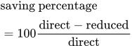 LaTeX:
\mathrm{saving\ percentage}=100\frac{\mathrm{direct}-\mathrm{reduced}}{\mathrm{direct}}Yaad rakhne ka cue: Har output cell ka kaam × kitne output cells.
Solution — step by step
Meaning and formula
A MAC is one multiply–accumulate operation. For the convention used here, count the weight–input products over every output location. Bias additions are omitted. A 1 × 1 bottleneck reduces channels before the expensive 3 × 3 layer.
LaTeX: \mathrm{MACs}=H_{\mathrm{out}}W_{\mathrm{out}}C_{\mathrm{out}}K^2C_{\mathrm{in}}Step 1: direct 3 × 3 convolution
Each output uses 3 × 3 × 64 = 576 weight–input pairs. There are 16 × 16 × 32 = 8,192 outputs.
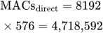 LaTeX:
\mathrm{MACs}_{\mathrm{direct}}=8192\times576=4{,}718{,}592Step 2: 1 × 1 reduction from 64 to 8 channels
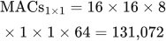 LaTeX:
\mathrm{MACs}_{1\times1}=16\times16\times8\times1\times1\times64=131{,}072Step 3: 3 × 3 convolution now receives only 8 channels
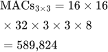 LaTeX:
\mathrm{MACs}_{3\times3}=16\times16\times32\times3\times3\times8=589{,}824Step 4: add the two bottleneck stages
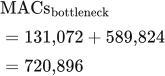 LaTeX:
\mathrm{MACs}_{\mathrm{bottleneck}}=131{,}072+589{,}824=720{,}896Step 5: calculate the saving
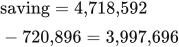 LaTeX:
\mathrm{saving}=4{,}718{,}592-720{,}896=3{,}997{,}696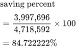 LaTeX:
\mathrm{saving\ percent}=\frac{3{,}997{,}696}{4{,}718{,}592}\times100=84.722222\%Final answer: direct 4,718,592 MACs; bottleneck 720,896 MACs; approximately 84.72% fewer. The output shape stays 16 × 16 × 32.
Bottleneck computation on an 8 × 8 input
Question. An 8 × 8 × 16 input must produce 8 channels using a same-padded 3 × 3 convolution. Compare direct computation with 1 × 1 reduction to 4 channels followed by the 3 × 3 layer. Count MACs and ignore bias additions.
Given
Spatial output = 8 × 8 in both stages.
Input channels = 16; output filters = 8; main kernel = 3 × 3.
Bottleneck uses 4 filters of 1 × 1.
To find
Direct MACs, two-stage bottleneck MACs and savings.
Formula — which one and why
Each output scalar requires one multiply-accumulate per incoming kernel entry. A bottleneck reduces the input depth of the expensive spatial convolution.
One MAC is one multiply-accumulate pair. If counting multiplication and addition separately, the operation count is approximately twice the MAC count.
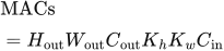 LaTeX:
\mathrm{MACs}=H_{\mathrm{out}}W_{\mathrm{out}}C_{\mathrm{out}}K_hK_wC_{\mathrm{in}}Yaad rakhne ka cue: Spatial kernel se pehle channels kam; dono stages ka cost add.
Solution — step by step
Step 1: count output positions per channel.
 LaTeX:
8(8)=64Step 2: count direct work per output scalar.
 LaTeX:
3(3)(16)=144Step 3: count the full direct layer.
 LaTeX:
64(8)(144)=73728Step 4: count the 1 × 1 reduction.
 LaTeX:
64(4)(1)(1)(16)=4096Step 5: count the reduced-depth 3 × 3 layer.
 LaTeX:
64(8)(3)(3)(4)=18432Step 6: sum both bottleneck stages.
LaTeX: 4096+18432=22528Step 7: subtract to obtain savings.
LaTeX: 73728-22528=51200Final answer: Direct = 73,728 MACs; bottleneck = 22,528 MACs; savings = 51,200 MACs.
Concatenation and residual addition
Concatenation and addition combine branches differently. Concatenation places channel groups next to each other and increases the channel count. Residual addition adds matching entries, so the two full shapes must be compatible.
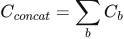 LaTeX:
C_{concat}=\sum_b C_b LaTeX:
y_{res}=F(x)+xInception concatenation and residual addition
Definition. Channel concatenation joins feature tensors while preserving their separate channels. Residual addition sums corresponding entries. These operations impose different shape constraints and produce different output depths.
Explanation and working
Concatenation joins feature channels; elementwise addition sums matching entries. They are different operations.
Four Inception branches of spatial size 14 × 14 have 16, 32, 8 and 8 channels. First add the channel counts: 16 + 32 = 48; 48 + 8 = 56; 56 + 8 = 64. Height and width stay 14. The concatenated output is 14 × 14 × 64.
A residual addition requires matching shapes. A 14 × 14 × 64 tensor cannot be directly added to a 14 × 14 × 32 tensor. A projection, often a 1 × 1 convolution, can transform one path to the matching shape before addition.
ResNet adds a shortcut
Definition. A residual network uses shortcut connections to learn a residual mapping relative to a block's input. A basic residual block adds the block transformation F(x) to a shortcut representation of x.
 LaTeX:
y=F(x)+xIf the desired mapping is H(x), the residual branch represents F(x) = H(x) − x. When the useful mapping is close to identity, a small residual can be easier to optimize than reconstructing identity through the entire branch.
Effect on gradient propagation
For the identity-shortcut formulation, the derivative includes a direct identity contribution.
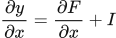 LaTeX:
\frac{\partial y}{\partial x}=\frac{\partial F}{\partial x}+IThis provides a path for information and derivatives that does not require passing through every weight layer in the residual branch. It helps optimize deep networks and addresses the degradation problem. It does not imply that every possible ResNet is immune to vanishing gradients.
Projection when dimensions differ
If channels or spatial dimensions change, use a projection shortcut, often a 1 × 1 convolution with suitable stride.
 LaTeX:
y=F(x)+W_sxAn identity shortcut has no learned parameters. A projection does. For Cᵢ input channels and Cₒ output channels, a biased 1 × 1 projection has CᵢCₒ + Cₒ parameters. The residual branch's output must match the projection output for addition.
Question. Let x = [1, 2, 3] and F(x) = [0.1, −0.2, 0.3]. Find the residual sum.
Given
x = [1,2,3]; residual branch F(x) = [0.1,−0.2,0.3].
To find
Find the three components of x+F(x).
Formula — which one and why
Residual addition. Add corresponding components of the input shortcut and learned branch. Apply the output activation afterward if requested.
x = shortcut/input; F(x) = residual branch output. Both arrays must have matching shapes before addition.
 LaTeX:
y=x+F(x)Yaad rakhne ka cue: Same position ke numbers add; shape same rehni chahiye.
Solution — step by step
Step 1: add the first matching pair.
 LaTeX:
1+0.1=1.1Step 2: add the second matching pair.
 LaTeX:
2+(-0.2)=1.8Step 3: add the third matching pair.
 LaTeX:
3+0.3=3.3Step 4: assemble in the original order.
 LaTeX:
y=[1.1,1.8,3.3]The vector length remains 3. Concatenating these vectors would give length 6 and would implement a different operation. Any post-addition activation specified in the architecture is applied after this sum.
Drill 44 Inception concatenation and parameter count
Question
Question. Input 10 × 10 × 8. Parallel branches: A uses 1 × 1 conv 4 filters ; B uses 3 × 3 same Conv 6 filters; C max pool 3 same, stride 1 then 1 × 1 conv 2 filters. Find combined shape and trainable parameters.
Answer — step by step
Given
Input = 10 × 10 × 8.
Branch A: 1 × 1 convolution, 4 filters.
Branch B: 3 × 3 same convolution, 6 filters.
Branch C: 3 × 3 same max pool with stride 1, then 1 × 1 convolution, 2 filters.
To find
Find each branch shape and parameters, then the concatenated shape and total parameters.
Formula — which one and why
Inception channel concatenation. Parallel branches retain their separate features. Add their channel counts while keeping the common height and width. Add trainable parameters across branches.
C₁,C₂,… = branch output channels. Concatenation requires matching spatial dimensions.
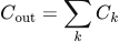 LaTeX:
C_{\mathrm{out}}=\sum_k C_k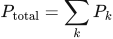 LaTeX:
P_{\mathrm{total}}=\sum_k P_kYaad rakhne ka cue: Channels jodo; height-width same rakho.
Convolution parameters. Every filter spans all input channels. Count its spatial coefficients across those channels, add one bias and multiply by the number of filters.
K_h,K_w = filter height/width; C_in = input channels; C_out = number of filters and output channels. Spatial output positions reuse these weights.
LaTeX: N_w=K_hK_wC_{\mathrm{in}}C_{\mathrm{out}}LaTeX: N_b=C_{\mathrm{out}}LaTeX: P=N_w+N_bYaad rakhne ka cue: Filter area × input channels × filters; phir ek bias per filter.
Solution — step by step
Meaning and formulas
Each parallel branch receives the same original 10 × 10 × 8 input. “Same” with stride 1 preserves height and width. Concatenation joins the channel lists without adding the feature values.
 LaTeX:
C_{\mathrm{combined}}=C_A+C_B+C_CLaTeX: P_{\mathrm{conv}}=(K^2C_{\mathrm{in}}+1)C_{\mathrm{out}}Assume one bias per filter. Pooling has no learned parameters.
Step 1: Branch A.
Its 4 filters produce shape 10 × 10 × 4.
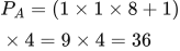 LaTeX:
P_A=(1\times1\times8+1)\times4=9\times4=36Step 2: Branch B.
Its 6 filters produce shape 10 × 10 × 6.
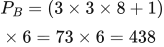 LaTeX:
P_B=(3\times3\times8+1)\times6=73\times6=438Step 3: Branch C.
Pooling preserves 10 × 10 × 8 here because stride is 1 and padding is same. Its parameter count is zero. The following 2-filter projection creates 10 × 10 × 2.
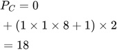 LaTeX:
P_C=0+(1\times1\times8+1)\times2=18Step 4: Join the shapes and add the parameters.
 LaTeX:
C_{\mathrm{combined}}=4+6+2=12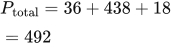 LaTeX:
P_{\mathrm{total}}=36+438+18=492Final answer: combined shape 10 × 10 × 12; 492 parameters. Branch B does not take branch A's four channels as input: they are parallel branches.
Drill 45 Projection shortcut
Question
Question. A residual main path outputs 8 × 8 × 16 but input is 16 × 16 × 8. Design a 1 × 1 projection shortcut with stride 2, zero padding. Find its output and parameters.
Answer — step by step
Given
Residual input = 16 × 16 × 8; main-path output = 8 × 8 × 16.
Shortcut kernel = 1 × 1; stride 2; padding 0.
Use one bias per projection filter.
To find
Choose the number of filters and find projection output shape and parameters.
Formula — which one and why
Convolution/pooling spatial size. Padding adds P positions at both ends. Subtract kernel width to find the last valid start, divide by stride, take the floor and include the initial placement with +1.
N = current height or width; K = kernel/window size; S = stride; P = padding per side. Apply separately to height and width; dilation is 1 here.
LaTeX: N_{\mathrm{out}}=\left\lfloor\frac{N+2P-K}{S}\right\rfloor+1Yaad rakhne ka cue: Input + dono sides ki padding − kernel; stride se divide; floor + 1.
Convolution parameters. Every filter spans all input channels. Count its spatial coefficients across those channels, add one bias and multiply by the number of filters.
K_h,K_w = filter height/width; C_in = input channels; C_out = number of filters and output channels. Spatial output positions reuse these weights.
LaTeX: N_w=K_hK_wC_{\mathrm{in}}C_{\mathrm{out}}LaTeX: N_b=C_{\mathrm{out}}LaTeX: P=N_w+N_bYaad rakhne ka cue: Filter area × input channels × filters; phir ek bias per filter.
Solution — step by step
Meaning and formulas
Residual addition needs identical shapes on both paths. The projection must reduce height and width from 16 to 8 and increase channels from 8 to 16.
LaTeX: N_{\mathrm{out}}=\left\lfloor\frac{N+2P-K}{S}\right\rfloor+1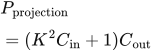 LaTeX:
P_{\mathrm{projection}}=(K^2C_{\mathrm{in}}+1)C_{\mathrm{out}}Step 1: choose 16 filters
One filter creates one channel, so 16 filters give the required 16 output channels.
Step 2: use the specified 1 × 1 kernel and stride 2
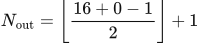 LaTeX:
N_{\mathrm{out}}=\left\lfloor\frac{16+0-1}{2}\right\rfloor+1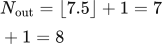 LaTeX:
N_{\mathrm{out}}=\lfloor7.5\rfloor+1=7+1=8The floor operation drops the fractional part; it does not round 7.5 to 8 before adding 1.
Step 3: count weights and biases
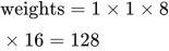 LaTeX:
\text{weights}=1\times1\times8\times16=128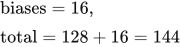 LaTeX:
\text{biases}=16,\qquad \text{total}=128+16=144Final answer: projection output 8 × 8 × 16 and 144 parameters with biases. The projected shortcut now matches the main path, so elementwise addition is valid.
Drill 38 Residual addition
Question
Question. x = [2,−3,1], F(x) = [−1,1,0.5]. Calculate residual output before and after ReLU and compare the plain block.
Answer — step by step
Given
x = [2,−3,1]; F(x) = [−1,1,0.5].
To find
Find x+F(x), apply ReLU, and compare with ReLU(F(x)).
Formula — which one and why
Residual addition. Add corresponding components of the input shortcut and learned branch. Apply the output activation afterward if requested.
x = shortcut/input; F(x) = residual branch output. Both arrays must have matching shapes before addition.
LaTeX: y=x+F(x)Yaad rakhne ka cue: Same position ke numbers add; shape same rehni chahiye.
ReLU and Leaky ReLU. ReLU returns zero for negative input and retains positive input. Leaky ReLU instead multiplies a negative input by its supplied slope.
z = preactivation; α (alpha) = supplied negative-side slope for Leaky ReLU. The derivative at zero needs an explicit convention.
LaTeX: \operatorname{ReLU}(z)=\max(0,z)LaTeX: \operatorname{LeakyReLU}(z)=\begin{cases}z&z\ge0\\\alpha z&z<0\end{cases}Yaad rakhne ka cue: Positive ko rehne do; negative ko zero. Leaky mein chhota negative rehne do.
Solution — step by step
Meaning and formulas
The main branch produces F(x). The shortcut carries x. A residual join adds matching entries from these equally sized vectors. ReLU is a separate operation after that join.
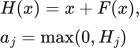 LaTeX:
H(x)=x+F(x),\qquad a_j=\max(0,H_j)Step 1: add each pair
 LaTeX:
H_1=2+(-1)=1 LaTeX:
H_2=-3+1=-2 LaTeX:
H_3=1+0.5=1.5The residual output before ReLU is [1, −2, 1.5].
Step 2: apply ReLU
 LaTeX:
[\max(0,1),\max(0,-2),\max(0,1.5)]=[1,0,1.5]Step 3: compare with the plain branch
Without a shortcut, the raw output is just F(x) = [−1, 1, 0.5]. Its ReLU output is [0, 1, 0.5].
Residual addition keeps three entries. Concatenation would join the vectors into six entries and is a different operation.
Batch normalization and learned scale/shift
Batch normalization first uses batch statistics, then applies a learned scale and shift. Epsilon belongs inside the square root. Inference ordinarily uses stored running statistics.
LaTeX: \mu_B=\frac{1}{m}\sum_{i=1}^{m}x_iLaTeX: \sigma_B^2=\frac{1}{m}\sum_{i=1}^{m}(x_i-\mu_B)^2LaTeX: \hat{x}_i=\frac{x_i-\mu_B}{\sqrt{\sigma_B^2+\epsilon}}LaTeX: y_i=\gamma\hat{x}_i+\betaBatch normalization inside a residual network
Definition. Batch normalization normalizes a feature using training-batch statistics, then applies a learned scale and shift. It operates on intermediate activations and is different from normalizing the original dataset once before training.
For one feature with m values in a training batch:
LaTeX: \mu_B=\frac{1}{m}\sum_{i=1}^{m}x_iLaTeX: \sigma_B^2=\frac{1}{m}\sum_{i=1}^{m}(x_i-\mu_B)^2LaTeX: \hat{x}_i=\frac{x_i-\mu_B}{\sqrt{\sigma_B^2+\epsilon}}LaTeX: y_i=\gamma\hat{x}_i+\betaThe batch mean μ_B is the centre; batch variance σ²_B measures squared spread. Epsilon ε is a small positive stability constant inside the square root. Gamma γ is a learned scale and beta β is a learned shift. For convolutional BN, statistics are usually computed separately for each channel across batch and spatial positions. Ordinary inference uses stored running statistics rather than the current test batch.
Question (practice, 3 marks). For one feature, a training batch contains [2,4]. Use ε = 0.00001, γ = 2 and β = 0.5. Calculate both batch-normalized outputs using population variance.
Given
x₁ = 2; x₂ = 4; m = 2; ε = 0.00001; γ = 2; β = 0.5.
To find
Batch mean, variance, normalized values and scale-and-shift outputs.
Formula — which one and why
Use the four formulas above in order. Population variance divides by m = 2, not m − 1. Scale and shift follow normalization because the model can learn the useful final feature scale.
Solution — step by step
Step 1: mean.
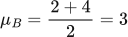 LaTeX:
\mu_B=\frac{2+4}{2}=3Step 2: deviations. 2 − 3 = −1 and 4 − 3 = 1.
Step 3: squared deviations and variance.
 LaTeX:
\sigma_B^2=\frac{(-1)^2+1^2}{2}=\frac{1+1}{2}=1Step 4: stable denominator.
 LaTeX:
d=\sqrt{1+0.00001}\approx1.00000499999Step 5: normalize separately.
 LaTeX:
\hat{x}_1=\frac{-1}{d}\approx-0.99999500004 LaTeX:
\hat{x}_2=\frac{1}{d}\approx0.99999500004Step 6: scale the first normalized value, then shift it.
 LaTeX:
y_1=2(-0.99999500004)+0.5\approx-1.49999000008Step 7: scale the second normalized value, then shift it.
 LaTeX:
y_2=2(0.99999500004)+0.5\approx2.49999000008Final answer: output ≈ [−1.49999,2.49999]. Its mean is β = 0.5; the final output need not have zero mean after the learned shift. The normalized values themselves have mean zero here.
Yaad rakho: centre hatao → spread se divide → learned scale lagao → shift add karo.
Global average pooling
Global average pooling takes one mean per complete spatial channel. The worked example compares the resulting dense classifier with a classifier after flattening.
LaTeX: g_c=\frac{1}{HW}\sum_{i=1}^{H}\sum_{j=1}^{W}a_{i,j,c}Global average pooling: one average for each channel
Definition. Global average pooling, or GAP, replaces every complete spatial feature map by its mean. An H × W × C tensor becomes C numbers. The channels remain separate; we do not average all channels into one number.
LaTeX: g_c=\frac{1}{HW}\sum_{i=1}^{H}\sum_{j=1}^{W}a_{i,j,c}The letter c selects a channel; i and j select its row and column; a is the value at that location. Add all H × W entries in that channel and divide by H × W. GAP has no learned weights or biases. A classifier after GAP can still have trainable parameters. In GoogLeNet, 7 × 7 × 1,024 becomes 1 × 1 × 1,024 before the final 1,000-class linear classifier.
Question (practice, 3 marks). A 2 × 2 × 2 tensor has channel A =  LaTeX:
\begin{bmatrix}1 & 3\\5 & 7\end{bmatrix} and channel B =  LaTeX:
\begin{bmatrix}2 & 4\\6 & 8\end{bmatrix}. Apply GAP, then find the parameters of a three-output dense classifier receiving the result, including one bias per output.
Given
H = 2, W = 2, C = 2. Each of the two channels contains four values. The classifier has three outputs.
To find
The GAP result and dense-head parameter count.
Formula — which one and why
Use one mean per channel. The dense layer receives two numbers, so each of its three outputs needs two weights and one bias.
LaTeX: P_{\mathrm{dense}}=(n_{\mathrm{in}}+1)n_{\mathrm{out}}Solution — step by step
Step 1: add channel A. 1 + 3 + 5 + 7 = 16.
Step 2: average channel A. 16 ÷ 4 = 4.
Step 3: add channel B. 2 + 4 + 6 + 8 = 20.
Step 4: average channel B. 20 ÷ 4 = 5. Thus GAP outputs [4,5].
Step 5: count the classifier's weights. 2 inputs × 3 outputs = 6 weights.
Step 6: add three biases. 6 + 3 = 9 parameters. GAP itself contributes zero.
Final answer: GAP = [4,5]; GAP shape = 1 × 1 × 2; classifier parameters = 9. If we flattened all eight inputs instead, that head would require (8 + 1) × 3 = 27 parameters.
Yaad rakho: ek channel ka poora average; channels ko aapas mein mat milao.
Top-k error percentage
Top-k error counts examples whose correct class is absent from the highest-scoring k predictions. Success counts must not be added twice.
LaTeX: E_k=\frac{N-C_k}{N}\times100\%Top-1 and top-5 error: what an ImageNet result means
Top-1 prediction is the class with the highest score. A top-1 mistake occurs when that class is wrong. Top-5 prediction is the list of the five highest-scoring classes. A top-5 mistake occurs only when the correct class is absent from that list. It is not the average error of five separate models.
For an image of a cat, the ordered list dog, cat, fox, horse, bird is a top-1 error but a top-5 success. The ordered list dog, fox, horse, bird, car is an error under both measures.
Question (practice, 2 marks). A classifier evaluates 100 images. The correct class is ranked first for 78 images and appears somewhere in the first five positions for 92 images. Calculate top-1 error and top-5 error.
Given
Total images = 100; top-1 successes = 78; top-5 successes = 92. The 78 first-place successes are already included in the 92 top-five successes.
To find
The percentage of mistakes under each rule.
Formula — which one and why
Subtract successful images from the total to obtain mistakes. Divide mistakes by the total and multiply by 100 to express a percentage.
LaTeX: E_k=\frac{N-C_k}{N}\times100\%N means total evaluated images; C_k means images whose correct class appears among the top k predictions.
Solution — step by step
Step 1: top-1 mistakes. 100 − 78 = 22.
Step 2: top-1 error percentage.
 LaTeX:
E_1=\frac{22}{100}\times100\%=22\%Step 3: top-5 mistakes. 100 − 92 = 8.
Step 4: top-5 error percentage.
 LaTeX:
E_5=\frac{8}{100}\times100\%=8\%Final answer: top-1 error = 22%; top-5 error = 8%. A broader acceptable list makes top-5 error no greater than top-1 error for the same evaluated predictions.
Yaad rakho: top-five mein sahi naam mil gaya toh top-five success.