Deep Learning · MT2 · section
Loss: how one wrong prediction becomes a number
Mathematics revision
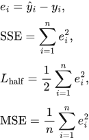
Definition. A residual is the signed prediction error. Squared-error objectives aggregate squared residuals; their scaling convention changes both the reported loss and its derivative.
 LaTeX:
e_i=\hat y_i-y_i,\qquad \mathrm{SSE}=\sum_{i=1}^{n}e_i^2,\qquad L_{\mathrm{half}}=\frac12\sum_{i=1}^{n}e_i^2,\qquad \mathrm{MSE}=\frac1n\sum_{i=1}^{n}e_i^2For this definition of n, each i indexes one included scalar prediction. In a multi-output batch, state whether the mean is over examples, output coordinates, or both. Half SSE and MSE happen to agree when n = 2; they are not generally the same objective.
Derivatives and their scaling
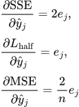
When differentiating with respect to prediction j, all other prediction terms are constant. The derivative of the j-th square is twice its residual:
 LaTeX:
\frac{\partial\mathrm{SSE}}{\partial\hat y_j}=2e_j,\qquad \frac{\partial L_{\mathrm{half}}}{\partial\hat y_j}=e_j,\qquad \frac{\partial\mathrm{MSE}}{\partial\hat y_j}=\frac{2}{n}e_jThe factor 1/2 cancels the derivative's factor 2. The factor 1/n instead produces 2/n. A weight derivative must also multiply by the derivative of the prediction with respect to that weight.
Question. Predictions are [0.2, 0.7, 0.4] and targets are [0, 1, 1]. Find SSE, half SSE and MSE, then their gradients with respect to the prediction vector.
Given
Predictions = [0.2,0.7,0.4].
Targets = [0,1,1]; n = 3 scalar predictions.
To find
Find SSE, half SSE and MSE, then all three prediction-gradient lists.
Formula — which one and why
Squared-error objectives. Calculate signed errors first and square them. SSE adds the squares; half SSE divides that sum by 2; MSE divides by the number of scalar predictions. These denominators are different conventions.
ŷᵢ = prediction; yᵢ = target; eᵢ = signed error; n = number of scalar predictions included in the stated loss.
 LaTeX:
e_i=\hat y_i-y_i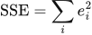 LaTeX:
\mathrm{SSE}=\sum_i e_i^2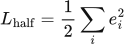 LaTeX:
L_{\mathrm{half}}=\frac12\sum_i e_i^2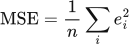 LaTeX:
\mathrm{MSE}=\frac1n\sum_i e_i^2Yaad rakhne ka cue: Pehle error square; phir question ke hisaab se sum, half ya mean.
Solution — step by step
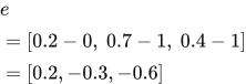
Step 1: calculate the three signed prediction errors.
 LaTeX:
e=[0.2-0,\ 0.7-1,\ 0.4-1]=[0.2,-0.3,-0.6]Step 2: square every error.
 LaTeX:
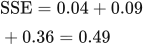
e\odot e=[0.04,0.09,0.36]Step 3: add the three squared errors.
 LaTeX:
\mathrm{SSE}=0.04+0.09+0.36=0.49Step 4: apply the requested loss divisors.
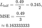 LaTeX:
L_{\mathrm{half}}=\frac{0.49}{2}=0.245,\qquad \mathrm{MSE}=\frac{0.49}{3}\approx0.163333333Step 5: multiply every error by 2 for the SSE gradient.
 LaTeX:
\nabla_{\hat y}\mathrm{SSE}=[0.4,-0.6,-1.2]Step 6: use each error itself for the half-SSE gradient.
 LaTeX:
\nabla_{\hat y}L_{\mathrm{half}}=[0.2,-0.3,-0.6]Step 7: multiply every error by 2/3 for the MSE gradient.
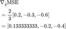 LaTeX:
\nabla_{\hat y}\mathrm{MSE}=\frac23[0.2,-0.3,-0.6]=[0.133333333,-0.2,-0.4]The residual signs survive in the gradients even though the losses are nonnegative. Multiplying a loss by a positive constant leaves its unregularized minimizers unchanged, but scales its gradients and therefore its updates at a fixed learning rate.