Deep Learning · MT2 · section
Probability mean and variance in plain language
The maths behind a network
Definitions. A probability assigns a value between 0 and 1 to an event. A discrete probability distribution assigns probabilities to mutually exclusive outcomes whose probabilities sum to 1. Expectation is a probability-weighted average. Variance measures expected squared deviation from the mean.
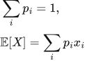 LaTeX:
\sum_i p_i=1,\qquad\mathbb E[X]=\sum_i p_i x_i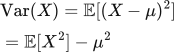 LaTeX:
\operatorname{Var}(X)=\mathbb E[(X-\mu)^2]=\mathbb E[X^2]-\mu^2Conditional probability and classification
P(A|B) is the probability of A conditional on B, defined when P(B) > 0. Bayes' rule relates it to the reverse conditional probability.
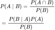 LaTeX:
P(A\mid B)=\frac{P(A\cap B)}{P(B)}=\frac{P(B\mid A)P(A)}{P(B)}For classification, the network estimates P(class | input). A softmax output is normalized across mutually exclusive classes. Independent sigmoid outputs are used for multiple labels that can be present together.
Empirical mean, variance and standardization
For N observed values, use the stated variance convention. These notes use division by N for the population-style variance in the numerical; an unbiased sample-variance estimate uses N − 1.
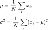 LaTeX:
\mu=\frac1N\sum_i x_i,\qquad\sigma^2=\frac1N\sum_i(x_i-\mu)^2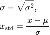 LaTeX:
\sigma=\sqrt{\sigma^2},\qquad x_{\mathrm{std}}=\frac{x-\mu}{\sigma}For values [3, 3, 7, 7], μ = 5, squared deviations are [4, 4, 4, 4], σ² = 16/4 = 4 and σ = 2. Thus a value 7 standardizes to (7 − 5)/2 = 1: one standard deviation above the mean. For preprocessing, fit μ and σ on training data and reuse them for validation/test data; σ must be nonzero.
Likelihood and cross-entropy
If the correct class has predicted probability p, its negative-log loss is −ln p. For p = 0.8, this is approximately 0.223144. For p = 0.1, it is approximately 2.302585. Increasing correct-class probability lowers this loss. Over independent examples, maximizing the product of correct-class probabilities is equivalent to minimizing the sum of negative log probabilities.
Population mean and spread: [1, 2, 3]
Question. For the population [1, 2, 3], find mean, population variance and standard deviation.
Given
Values = [1, 2, 3]; N = 3. Use population division by N.
To find
Mean μ, variance σ² and standard deviation σ.
Formula — which one and why
The question specifies a population, so use N rather than the N−1 sample-variance divisor.
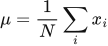
μ is the centre; σ² averages squared distances from it; σ converts spread back to the original units.
 LaTeX:
\mu=\frac1N\sum_i x_i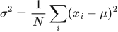 LaTeX:
\sigma^2=\frac1N\sum_i(x_i-\mu)^2 LaTeX:
\sigma=\sqrt{\sigma^2}Yaad rakhne ka cue: Mean, distance, square, mean again, then root.
Solution — step by step
Step 1: add all values.
 LaTeX:
1+2+3=6Step 2: divide by the number of values.
 LaTeX:
\mu=\frac{6}{3}=2Step 3: find and square deviation 1.
 LaTeX:
(1-2)=-1 LaTeX:
(-1)^2=1Step 4: find and square deviation 2.
 LaTeX:
(2-2)=0 LaTeX:
(0)^2=0Step 5: find and square deviation 3.
 LaTeX:
(3-2)=1 LaTeX:
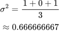
(1)^2=1Step 6: average the squared deviations.
 LaTeX:
\sigma^2=\frac{1+0+1}{3}\approx0.666666667Step 7: take the nonnegative square root.
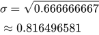 LaTeX:
\sigma=\sqrt{0.666666667}\approx0.816496581Final answer: μ = 2; σ² ≈ 0.666666667; σ ≈ 0.816496581.
Population mean and spread: [2, 2, 2]
Question. For the population [2, 2, 2], find mean, population variance and standard deviation.
Given
Values = [2, 2, 2]; N = 3. Use population division by N.
To find
Mean μ, variance σ² and standard deviation σ.
Formula — which one and why
The question specifies a population, so use N rather than the N−1 sample-variance divisor.
μ is the centre; σ² averages squared distances from it; σ converts spread back to the original units.
LaTeX: \mu=\frac1N\sum_i x_iLaTeX: \sigma^2=\frac1N\sum_i(x_i-\mu)^2LaTeX: \sigma=\sqrt{\sigma^2}Yaad rakhne ka cue: Mean, distance, square, mean again, then root.
Solution — step by step
Step 1: add all values.
 LaTeX:
2+2+2=6Step 2: divide by the number of values.
LaTeX: \mu=\frac{6}{3}=2Step 3: find and square deviation 1.
LaTeX: (2-2)=0LaTeX: (0)^2=0Step 4: find and square deviation 2.
LaTeX: (2-2)=0LaTeX: (0)^2=0Step 5: find and square deviation 3.
LaTeX: (2-2)=0LaTeX: (0)^2=0Step 6: average the squared deviations.
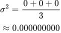 LaTeX:
\sigma^2=\frac{0+0+0}{3}\approx0.000000000Step 7: take the nonnegative square root.
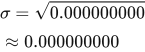 LaTeX:
\sigma=\sqrt{0.000000000}\approx0.000000000Final answer: μ = 2; σ² ≈ 0.000000000; σ ≈ 0.000000000. Standardization is undefined with this zero standard deviation.