Deep Learning · MT2 · section
What does learning from data mean
Neural-network foundations
Definition. Machine learning develops models from data so that they can perform a task on new examples. A model is a calculation rule with adjustable numbers. Deep learning uses neural networks with multiple trainable layers; each layer transforms the previous layer's outputs.
Start with one complete training example
A sample means one example in the dataset. Suppose one example says: an input number is 2 and the required answer is 4. We write the input as x = 2 and the correct answer, or target, as y = 4. These letters are labels for the two numbers.
An input feature is one recorded property used to make a prediction. One house might have area, number of rooms and age as three features. The three values together describe one sample. An input vector is just an ordered list of those feature values. Order matters: the first model weight must always multiply the first feature.
The model's calculated answer is the prediction, written ŷ, read “y hat”. The hat helps us distinguish the calculated answer ŷ from the required answer y. A prediction is a probability only when the task and output function give it that interpretation.
The simplest model: multiply, then add
In the following model, x is the input, w is a weight and b is a bias. A weight multiplies the input. A bias is added once after multiplication. Both w and b are adjustable model numbers, called parameters.
 LaTeX:
\hat y=wx+bThe model first multiplies w and x; then it adds b. For several inputs it uses one matching weight per input, adds their products, and then adds the bias.
Yaad rakhne ka cue: x diya hua input; y sahi answer; ŷ model ka answer; w aur b training mein badlenge.
Model example 1: calculate a prediction
Question. A linear model uses ŷ = wx+b. For x = 2, w = 1 and b = 0, calculate its prediction.
Given
Input x = 2.
Weight w = 1; bias b = 0.
The output is linear: no extra activation is specified.
To find
The predicted value ŷ.
Formula — which one and why
Use the stated model. The multiplication gives the input contribution; the bias shifts the result.
x is the input; w is its multiplier; b is the added offset; ŷ is the calculated output.
LaTeX: \hat y=wx+bYaad rakhne ka cue: Pehle input × weight, phir bias add.
Solution — step by step
Step 1: multiply the input by its weight.
 LaTeX:
wx=(1)(2)=2Step 2: add the bias once.
 LaTeX:
\hat y=2+(0)=2Final answer: ŷ = 2. This is a prediction, not a loss or a learned weight.
Model example 2: calculate a prediction
Question. A linear model uses ŷ = wx+b. For x = 2, w = 1.5 and b = 1, calculate its prediction.
Given
Input x = 2.
Weight w = 1.5; bias b = 1.
The output is linear: no extra activation is specified.
To find
The predicted value ŷ.
Formula — which one and why
Use the stated model. The multiplication gives the input contribution; the bias shifts the result.
x is the input; w is its multiplier; b is the added offset; ŷ is the calculated output.
LaTeX: \hat y=wx+bYaad rakhne ka cue: Pehle input × weight, phir bias add.
Solution — step by step
Step 1: multiply the input by its weight.
 LaTeX:
wx=(1.5)(2)=3Step 2: add the bias once.
 LaTeX:
\hat y=3+(1)=4Final answer: ŷ = 4. This is a prediction, not a loss or a learned weight.
Model example 3: calculate a prediction
Question. A linear model uses ŷ = wx+b. For x = 3, w = 1.5 and b = 1, calculate its prediction.
Given
Input x = 3.
Weight w = 1.5; bias b = 1.
The output is linear: no extra activation is specified.
To find
The predicted value ŷ.
Formula — which one and why
Use the stated model. The multiplication gives the input contribution; the bias shifts the result.
x is the input; w is its multiplier; b is the added offset; ŷ is the calculated output.
LaTeX: \hat y=wx+bYaad rakhne ka cue: Pehle input × weight, phir bias add.
Solution — step by step
Step 1: multiply the input by its weight.
 LaTeX:
wx=(1.5)(3)=4.5Step 2: add the bias once.
 LaTeX:
\hat y=4.5+(1)=5.5Final answer: ŷ = 5.5. This is a prediction, not a loss or a learned weight.
Model example 4: calculate a prediction
Question. A linear model uses ŷ = wx+b. For x = 2, w = -0.5 and b = 3, calculate its prediction.
Given
Input x = 2.
Weight w = -0.5; bias b = 3.
The output is linear: no extra activation is specified.
To find
The predicted value ŷ.
Formula — which one and why
Use the stated model. The multiplication gives the input contribution; the bias shifts the result.
x is the input; w is its multiplier; b is the added offset; ŷ is the calculated output.
LaTeX: \hat y=wx+bYaad rakhne ka cue: Pehle input × weight, phir bias add.
Solution — step by step
Step 1: multiply the input by its weight.
 LaTeX:
wx=(-0.5)(2)=-1Step 2: add the bias once.
 LaTeX:
\hat y=-1+(3)=2Final answer: ŷ = 2. This is a prediction, not a loss or a learned weight.
How the model learns
An initial model can predict 2 when the target is 4. A loss function measures the discrepancy. Training calculates how changing each parameter changes the loss; that rate is a gradient. An optimizer uses the gradient to adjust the parameters. The learning rate controls the size of this adjustment. The loss, derivative and complete update are explained with full examples in the next lessons.
The learning rate is a hyperparameter: a setting chosen for training. A learned weight is a parameter: an adjustable number inside the model. During ordinary inference, the trained weights stay fixed and the model calculates an output for a new input.
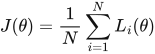
For many training samples, the objective normally averages the individual losses. θ (theta) means the collection of adjustable parameters; N is the number of training examples; Lᵢ is the loss for example i.
 LaTeX:
J(\theta)=\frac1N\sum_{i=1}^{N}L_i(\theta)Σ is an instruction to add the listed terms. For three losses it means L₁ + L₂ + L₃, followed by division by 3. Regularization may add a penalty; the regularization chapter explains that separate term.
Why several layers help
A layer contains several neurons that calculate outputs from the same incoming values. In an image model, earlier layers can respond to simple patterns such as edges; later layers combine earlier responses into more complex features. This hierarchy is learned from data. A deep network is not guaranteed to learn useful features merely because it has many layers; training data, architecture and optimization still matter.
Generalization means performing well on new examples. Training data adjusts weights; validation data helps choose settings and stopping time; held-out test data evaluates the chosen model. Small training loss alone does not establish good generalization.
Yaad rakhne ka cue: training = answer nikalo → loss nikalo → gradients nikalo → parameters update karo; inference = trained model se answer nikalo.
Average training loss
Question. Three training examples have losses 2, 0.5 and 0.5. Calculate their mean training loss.
Given
L₁ = 2; L₂ = 0.5; L₃ = 0.5; N = 3.
To find
The mean loss J.
Formula — which one and why
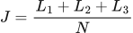
The question asks for the mean, so add all sample losses and divide by the number of samples.
Lᵢ means loss of example i. N counts examples.
 LaTeX:
J=\frac{L_1+L_2+L_3}{N}Yaad rakhne ka cue: Mean = total loss ÷ examples.
Solution — step by step
Step 1: add the losses.
 LaTeX:
2+0.5+0.5=3Step 2: divide by the number of examples.
 LaTeX:
J=\frac33=1Final answer: Mean training loss = 1.