Deep Learning · MT2 · section

Your first complete training step

Neural-network foundations

Question. A linear model is defined by LaTeX: \hat y=wx. For the training example x = 2, y = 4, use initial weight w₀ = 1, learning rate η = 0.1 and half squared loss. Perform two gradient-descent updates and report the prediction and loss after each update.

Given

Model: ŷ = wx; bias is absent and is not updated.

x = 2; y = 4; initial w₀ = 1; η = 0.1.

Loss = half squared error; perform two updates.

To find

Find the weight, prediction and loss after each update.

Formula — which one and why

Chain rule with only a trainable weight. The weight changes the prediction and the prediction changes the half squared loss. Multiply both rates, then subtract the scaled gradient. The stated model has no bias parameter.

ŷ = prediction; y = target; x = input; w = weight; η = learning rate; g = loss derivative with respect to w.

LaTeX: \hat y=wx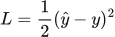

LaTeX: L=\frac12(\hat y-y)^2

LaTeX: g=(\hat y-y)x

LaTeX: w_{\mathrm{new}}=w-\eta g

Yaad rakhne ka cue: Prediction minus target, phir input se multiply; naya weight = purana − ηg.

Solution — step by step

Model, objective and gradient

The input and target remain fixed; only the weight is trainable. There is no bias parameter in this question.

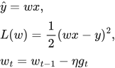LaTeX: \hat y=wx,\qquad L(w)=\frac12(wx-y)^2,\qquad w_t=w_{t-1}-\eta g_t

Apply the chain rule through the prediction:

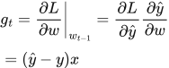LaTeX: g_t=\left.\frac{\partial L}{\partial w}\right|_{w_{t-1}}=\frac{\partial L}{\partial\hat y}\frac{\partial\hat y}{\partial w}=(\hat y-y)x

The factor 1/2 in the objective cancels the factor 2 from differentiating the square. The remaining factor x comes from differentiating wx with respect to w.

Visible text and connections in this diagram

HOW ONE WEIGHT LEARNS

1. PREDICT

Input x = 2

Weight w = 1

Prediction = 1 × 2 = 2

Target y = 4

Prediction is 2 too small.

2. MEASURE AND CORRECT

Loss = ½ × (2 − 4)² = 2

Gradient = (2 − 4) × 2 = −4

New weight = 1 − 0.1 × (−4) = 1.4

Learning rate = 0.1

3. PREDICT AGAIN

Same input x = 2

New weight w = 1.4

New prediction = 1.4 × 2 = 2.8

Target stays 4

Loss falls from 2 to 0.72.

Predict row: input to weight to prediction

Measure and correct row: loss to gradient to new weight

Predict again row: same input to new weight to new prediction

Diagram: Forward evaluation, gradient calculation and a parameter update for the same training example.

Iteration 1

Step 1: forward evaluation at the current parameter.

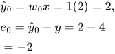LaTeX: \hat y_0=w_0x=1(2)=2,\qquad e_0=\hat y_0-y=2-4=-2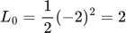

LaTeX: L_0=\frac12(-2)^2=2

Step 2: gradient at the current parameter.

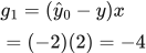LaTeX: g_1=(\hat y_0-y)x=(-2)(2)=-4

Step 3: parameter update.

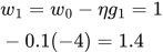LaTeX: w_1=w_0-\eta g_1=1-0.1(-4)=1.4

Step 4: evaluate the updated model.

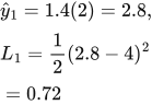LaTeX: \hat y_1=1.4(2)=2.8,\qquad L_1=\frac12(2.8-4)^2=0.72

Iteration 2

Use w₁ = 1.4 and recompute the gradient; reusing the previous gradient would not be gradient descent on this objective.

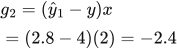LaTeX: g_2=(\hat y_1-y)x=(2.8-4)(2)=-2.4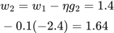

LaTeX: w_2=w_1-\eta g_2=1.4-0.1(-2.4)=1.64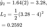

LaTeX: \hat y_2=1.64(2)=3.28,\qquad L_2=\frac12(3.28-4)^2=0.2592

Interpretation. Both gradients are negative, so the updates increase the weight toward the optimum w = y/x = 2. The loss decreases in these iterations. Gradient descent does not guarantee a decrease for every learning rate; step size matters.