Deep Learning · MT2 · section

More outputs and vectorized backpropagation

Neural-network foundations

Definition. Vectorized backpropagation expresses the chain rule using matrix products and elementwise derivatives. When a hidden activation affects several outputs, its derivative contains the sum of the contributions from every downstream path.

Why the hidden derivative is a sum

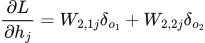
If hidden activation hⱼ connects to output preactivations zₒ₁ and zₒ₂, changing hⱼ changes both outputs. The multivariable chain rule gives:

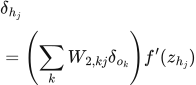
LaTeX: \frac{\partial L}{\partial h_j}=W_{2,1j}\delta_{o_1}+W_{2,2j}\delta_{o_2}

For any number of connected outputs, sum their contributions and then differentiate the hidden activation:

LaTeX: \delta_{h_j}=\left(\sum_k W_{2,kj}\delta_{o_k}\right)f'(z_{h_j})

Use the connecting weights from the original forward pass. Adding only the contribution of the first output would omit a dependency of the loss.

Diagram: The outgoing paths both contribute to the hidden derivative. Add the weighted output deltas, then apply the hidden activation derivative.. Labels: Two output paths both affect the hidden neuron | Two output paths both affect the hidden neuron | Example: hidden activation h = 0.6, using sigmoid in the hidden neuron. | h = 0.6 | Output 1 delta = 0.2 | Connecting weight = 0.4 | Output 2 delta = −0.1 | Connecting weight = 0.5 | Downstream sum = 0.2 × 0.4 + (−0.1) × 0.5 = 0.03 | Hidden delta = 0.03 × 0.6 × (1 − 0.6) = 0.0072 | Add the two downstream paths first. Then multiply by the hidden activation | derivative.

Matrix equations for one training sample

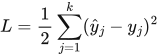
Use column vectors throughout. Let W₁ map d inputs to m hidden units and W₂ map those units to k outputs. The following output-delta formula assumes half sum of squared errors and an elementwise output activation f₂:

LaTeX: L=\frac12\sum_{j=1}^{k}(\hat y_j-y_j)^2

LaTeX: \delta_2=(\hat y-y)\odot f_2'(z_2)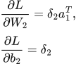

LaTeX: \frac{\partial L}{\partial W_2}=\delta_2a_1^T,\qquad\frac{\partial L}{\partial b_2}=\delta_2

LaTeX: \delta_1=(W_2^T\delta_2)\odot f_1'(z_1)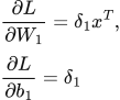

LaTeX: \frac{\partial L}{\partial W_1}=\delta_1x^T,\qquad\frac{\partial L}{\partial b_1}=\delta_1

Here ⊙ means elementwise multiplication. The product δ₂a₁ᵀ is an outer product: every receiving delta is multiplied by every sending activation.

How the loss changes the output delta

For MSE averaged over k output components, the squared-error derivative has the factor 2/k. For sigmoid with binary cross-entropy, or softmax with categorical cross-entropy and a normalized target, the paired derivative simplifies to prediction minus target:

LaTeX: \delta_{\mathrm{output}}=\hat y-y

That simplification already includes differentiation of the paired activation and loss. Multiplying by a sigmoid derivative again would be incorrect. For sigmoid with half squared error, the sigmoid derivative is still required.

For a batch, sum per-example parameter gradients; divide by the batch size only if the objective is a batch mean. State the output reduction and batch reduction separately when both appear in a question.