Deep Learning · MT2 · section
Complete sigmoid training example
Neural-network foundations
Question. A sigmoid neuron has input 2, weight 0, bias 0, target 1 and half squared loss. Will gradient descent increase or decrease the weight? Use learning rate 0.1 and calculate the exact update.
Given
x = 2; w = 0; b = 0; y = 1.
Sigmoid output; half squared loss; η = 0.1.
To find
Find the weight-gradient sign, exact weight update and resulting weight.
Formula — which one and why
Weighted sum and activation. Each input is multiplied by its connection weight. Add these contributions, add the bias once, then apply the stated activation.
xᵢ = input i; wᵢ = its weight; b = bias; z = sum before activation; a = output after activation; f = the specified activation function.
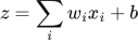 LaTeX:
z=\sum_iw_ix_i+b LaTeX:
a=f(z)Yaad rakhne ka cue: Input × weight, sabka sum, bias once, phir activation.
Sigmoid and its slope. Use sigmoid when the neuron is specified to squash its preactivation into (0,1). Once its output is known, its derivative needs only output × (1−output).
z = preactivation; p = sigmoid output; e is the exponential base, not a prediction error in this formula.
 LaTeX:
p=\frac{1}{1+e^{-z}}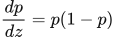 LaTeX:
\frac{dp}{dz}=p(1-p)Yaad rakhne ka cue: Sigmoid output p; uska slope p × (1−p).
Half summed squared loss. This loss convention takes one-half of the sum of squared prediction errors. Use it when the question specifies it, or explicitly state it as an assumption when the paper omits the loss. Differentiating cancels the factor one-half against the square derivative.
oⱼ = output j; yⱼ = target j; L = half summed squared loss under the stated or explicitly assumed convention.
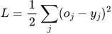 LaTeX:
L=\frac12\sum_j(o_j-y_j)^2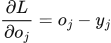 LaTeX:
\frac{\partial L}{\partial o_j}=o_j-y_jYaad rakhne ka cue: Half aur square ka 2 cancel: output derivative = prediction − target.
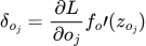
Backpropagation. The loss tells us how each output must change. Multiply by that neuron’s activation slope to obtain its delta. A weight gradient is receiving delta × sending value. Hidden deltas must include every outgoing path.
δ (delta) = derivative of loss with respect to a neuron’s preactivation; f′ = activation derivative; aᵢ = sending activation; Wⱼᵢ = connection weight. Use the exact loss scaling in the question.
 LaTeX:
\delta_{o_j}=\frac{\partial L}{\partial o_j}f_o\prime(z_{o_j})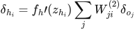 LaTeX:
\delta_{h_i}=f_h\prime(z_{h_i})\sum_jW_{ji}^{(2)}\delta_{o_j}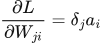 LaTeX:
\frac{\partial L}{\partial W_{ji}}=\delta_ja_i LaTeX:
\frac{\partial L}{\partial b_j}=\delta_j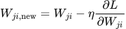 LaTeX:
W_{ji,\mathrm{new}}=W_{ji}-\eta\frac{\partial L}{\partial W_{ji}}Yaad rakhne ka cue: Receiving delta × sending value = us connection ka gradient.
Solution — step by step
Step 1 forward: net = 0(2) + 0 = 0; sigmoid output = 0.5.
Step 2 backward: prediction minus target = 0.5 − 1 = −0.5. Sigmoid slope = 0.5(1 − 0.5) = 0.25. Delta = −0.5 × 0.25 = −0.125.
Step 3 gradients and update: weight gradient = −0.125 × 2 = −0.25. New weight = 0 − 0.1(−0.25) = 0.025. Bias gradient = −0.125; new bias = 0.0125. Both increase. With positive input, these changes initially raise the prediction toward the target. Your intuition and arithmetic now agree.