Deep Learning · MT2 · section
Choosing a loss
Neural-network foundations
Definition. A loss function quantifies the discrepancy between a prediction and its target. The training objective aggregates per-example losses and may add regularization. The loss must be compatible with the task and output parameterization.
Explanation and working
Activation produces the prediction. Loss measures how wrong that prediction is. An optimizer uses gradients to update parameters. These are three different roles.
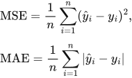 LaTeX:
\operatorname{MSE}=\frac1n\sum_{i=1}^n(\hat y_i-y_i)^2,\qquad \operatorname{MAE}=\frac1n\sum_{i=1}^n|\hat y_i-y_i|Question. Targets are [2, 4], predictions are [1, 6]. Find MSE and MAE.
Given
Targets = [2,4]; predictions = [1,6]; n = 2.
To find
Find mean squared error and mean absolute error.
Formula — which one and why
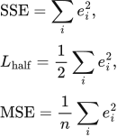
Squared-error objectives. Calculate signed errors first and square them. SSE adds the squares; half SSE divides that sum by 2; MSE divides by the number of scalar predictions. These denominators are different conventions.
ŷᵢ = prediction; yᵢ = target; eᵢ = signed error; n = number of scalar predictions included in the stated loss.
 LaTeX:
e_i=\hat y_i-y_i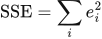 LaTeX:
\mathrm{SSE}=\sum_i e_i^2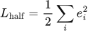 LaTeX:
L_{\mathrm{half}}=\frac12\sum_i e_i^2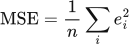 LaTeX:
\mathrm{MSE}=\frac1n\sum_i e_i^2Yaad rakhne ka cue: Pehle error square; phir question ke hisaab se sum, half ya mean.
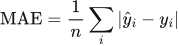
Mean absolute error. Absolute value removes the sign of each prediction error without squaring its magnitude. Average those magnitudes.
n = number of predictions. |e| means the nonnegative magnitude of error e.
 LaTeX:
\mathrm{MAE}=\frac1n\sum_i|\hat y_i-y_i|Yaad rakhne ka cue: MAE mein magnitude; MSE mein square.
Solution — step by step
Step 1: calculate prediction minus target.
 LaTeX:
e_1=1-2=-1 LaTeX:
e_2=6-4=2Step 2: square both errors.
 LaTeX:
e_1^2=(-1)^2=1 LaTeX:
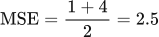
e_2^2=2^2=4Step 3: add squares and divide by two observations.
 LaTeX:
\mathrm{MSE}=\frac{1+4}{2}=2.5Step 4: take the absolute value of each original error.
 LaTeX:
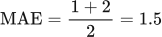
|-1|=1,\qquad |2|=2Step 5: add absolute errors and divide by two.
 LaTeX:
\mathrm{MAE}=\frac{1+2}{2}=1.5Final answer: MSE = 2.5; MAE = 1.5. Squaring gives larger errors more influence; MAE is not differentiable at zero error.
 LaTeX:
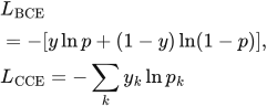
L_{\mathrm{BCE}}=-[y\ln p+(1-y)\ln(1-p)],\qquad L_{\mathrm{CCE}}=-\sum_k y_k\ln p_kFor binary y = 1, BCE becomes −ln(p). For y = 0, it becomes −ln(1 − p). For one-hot multiclass labels, CCE is simply minus the natural log of the predicted probability assigned to the correct class.
Question. True class is Mild, encoded [0,1,0], and probabilities are [0.1,0.8,0.1]. Find CCE.
Given
True class = Mild; one-hot target = [0,1,0].
Predicted probabilities = [0.1,0.8,0.1].
To find
Find the categorical cross-entropy.
Formula — which one and why
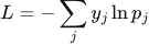
Categorical cross-entropy. For mutually exclusive classes with a one-hot target, all zero-target terms disappear. The loss is the negative log of the probability assigned to the true class.
yⱼ = target entry; pⱼ = predicted probability; c = index of the true class. Use natural logarithms unless another base is specified.
 LaTeX:
L=-\sum_j y_j\ln p_j LaTeX:
L=-\ln p_cYaad rakhne ka cue: One-hot mein sirf correct class ki probability ka minus ln.
Solution — step by step
Step 1: write one weighted log term for each class.
 LaTeX:
L=-[0\ln(0.1)+1\ln(0.8)+0\ln(0.1)]Step 2: remove terms with zero target weight.
 LaTeX:
L=-\ln(0.8)Step 3: evaluate the natural logarithm.
 LaTeX:
\ln(0.8)\approx-0.223143551Step 4: apply the outer minus sign.
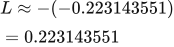 LaTeX:
L\approx-(-0.223143551)=0.223143551Final answer: CCE ≈ 0.223144. Only the correct-class probability contributes for this one-hot target.
| Task | Typical output | Typical loss |
|---|---|---|
| Unbounded numerical regression | One linear output | MSE or MAE |
| Binary classification | One sigmoid output | Binary cross-entropy |
| Exactly one of K classes | K softmax outputs | Categorical cross-entropy |
| Several independent labels | K sigmoid outputs | Binary cross-entropy per label |
A continuous rating restricted to 0–10 can use a linear output with a stated range policy, or 10 × sigmoid with an appropriate regression loss. If ratings are treated as discrete ordered categories, modelling choices differ. State the interpretation instead of selecting a loss merely from the number 10.
Squared-error scaling in backpropagation
For n included scalar predictions, let eᵢ = ŷᵢ−yᵢ. Three frequently used objectives are:
 LaTeX:
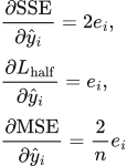
\mathrm{SSE}=\sum_i e_i^2,\qquad L_{\mathrm{half}}=\frac12\sum_i e_i^2,\qquad \mathrm{MSE}=\frac1n\sum_i e_i^2Differentiating with respect to one prediction produces different factors:
 LaTeX:
\frac{\partial\mathrm{SSE}}{\partial\hat y_i}=2e_i,\quad \frac{\partial L_{\mathrm{half}}}{\partial\hat y_i}=e_i,\quad \frac{\partial\mathrm{MSE}}{\partial\hat y_i}=\frac2n e_iUse the exact objective in the question. The teacher's two-output backpropagation example uses half SSE. Do not automatically insert the MSE factor into that example.
Why cross-entropy uses the negative logarithm
For a one-hot target, the likelihood of the observed class is the probability assigned to it. Maximizing that likelihood is equivalent to minimizing its negative logarithm. For independent training examples, multiplying probabilities becomes adding their logarithms. A low correct-class probability therefore produces a large loss.
Sigmoid with binary cross-entropy: output delta
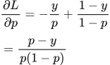
Let p = σ(z). First differentiate the loss with respect to p, holding y constant:
 LaTeX:
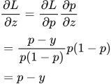
\frac{\partial L}{\partial p}=-\frac yp+\frac{1-y}{1-p}=\frac{p-y}{p(1-p)}Then multiply by the sigmoid derivative:
 LaTeX:
\frac{\partial L}{\partial z}=\frac{\partial L}{\partial p}\frac{\partial p}{\partial z}=\frac{p-y}{p(1-p)}p(1-p)=p-yThus the logit delta is p−y for this paired output and loss. With sigmoid and half squared error it is instead (p−y)p(1−p). Confusing these two cases changes every subsequent gradient.
Softmax with categorical cross-entropy: output delta
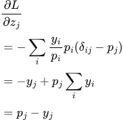
For a normalized target vector, the derivative of softmax component pᵢ with respect to logit zⱼ is pᵢ times (δᵢⱼ−pⱼ), where δᵢⱼ is 1 if i = j and 0 otherwise. Therefore:
 LaTeX:
\frac{\partial L}{\partial z_j}=-\sum_i\frac{y_i}{p_i}p_i(\delta_{ij}-p_j)=-y_j+p_j\sum_i y_i=p_j-y_jThis result assumes the target components sum to 1. For a mean loss over a batch, include the corresponding averaging factor as well.
Three squared-error conventions: [1, 3]
Question. Predictions are [1, 3] and targets are [2, 3]. Find SSE, half SSE and MSE.
Given
Predictions = [1, 3].
Targets = [2, 3].
Number of scalar predictions n = 2.
To find
SSE, half SSE and MSE separately.
Formula — which one and why
All three use the same squared errors but divide the sum differently. The question explicitly asks for each convention.
ŷᵢ is a prediction; yᵢ its target; n counts predictions, not network layers.
LaTeX: e_i=\hat y_i-y_iLaTeX: \mathrm{SSE}=\sum_i e_i^2LaTeX: L_{\mathrm{half}}=\frac12\sum_i e_i^2LaTeX: \mathrm{MSE}=\frac1n\sum_i e_i^2Yaad rakhne ka cue: Square sab mein; half mein 2, mean mein n se divide.
Solution — step by step
Step 1: calculate error 1.
LaTeX: e_1=1-2=-1Step 2: square error 1.
LaTeX: e_1^2=(-1)^2=1Step 3: calculate error 2.
 LaTeX:
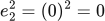
e_2=3-3=0Step 4: square error 2.
 LaTeX:
e_2^2=(0)^2=0Step 5: add squared errors.
 LaTeX:
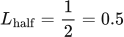
\mathrm{SSE}=1+0=1Step 6: divide by 2 for half SSE.
 LaTeX:
L_{\mathrm{half}}=\frac{1}{2}=0.5Step 7: divide by the number of predictions for MSE.
 LaTeX:
\mathrm{MSE}=\frac{1}{2}\approx0.500000000Final answer: SSE = 1; half SSE = 0.5; MSE ≈ 0.500000000.
Three squared-error conventions: [2, 5, 1]
Question. Predictions are [2, 5, 1] and targets are [1, 3, 2]. Find SSE, half SSE and MSE.
Given
Predictions = [2, 5, 1].
Targets = [1, 3, 2].
Number of scalar predictions n = 3.
To find
SSE, half SSE and MSE separately.
Formula — which one and why
All three use the same squared errors but divide the sum differently. The question explicitly asks for each convention.
ŷᵢ is a prediction; yᵢ its target; n counts predictions, not network layers.
LaTeX: e_i=\hat y_i-y_iLaTeX: \mathrm{SSE}=\sum_i e_i^2LaTeX: L_{\mathrm{half}}=\frac12\sum_i e_i^2LaTeX: \mathrm{MSE}=\frac1n\sum_i e_i^2Yaad rakhne ka cue: Square sab mein; half mein 2, mean mein n se divide.
Solution — step by step
Step 1: calculate error 1.
 LaTeX:
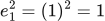
e_1=2-1=1Step 2: square error 1.
 LaTeX:
e_1^2=(1)^2=1Step 3: calculate error 2.
 LaTeX:
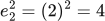
e_2=5-3=2Step 4: square error 2.
 LaTeX:
e_2^2=(2)^2=4Step 5: calculate error 3.
 LaTeX:
e_3=1-2=-1Step 6: square error 3.
 LaTeX:
e_3^2=(-1)^2=1Step 7: add squared errors.
 LaTeX:
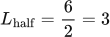
\mathrm{SSE}=1+4+1=6Step 8: divide by 2 for half SSE.
 LaTeX:
L_{\mathrm{half}}=\frac{6}{2}=3Step 9: divide by the number of predictions for MSE.
 LaTeX:
\mathrm{MSE}=\frac{6}{3}\approx2.000000000Final answer: SSE = 6; half SSE = 3; MSE ≈ 2.000000000.
Three squared-error conventions: [4]
Question. Predictions are [4] and targets are [1]. Find SSE, half SSE and MSE.
Given
Predictions = [4].
Targets = [1].
Number of scalar predictions n = 1.
To find
SSE, half SSE and MSE separately.
Formula — which one and why
All three use the same squared errors but divide the sum differently. The question explicitly asks for each convention.
ŷᵢ is a prediction; yᵢ its target; n counts predictions, not network layers.
LaTeX: e_i=\hat y_i-y_iLaTeX: \mathrm{SSE}=\sum_i e_i^2LaTeX: L_{\mathrm{half}}=\frac12\sum_i e_i^2LaTeX: \mathrm{MSE}=\frac1n\sum_i e_i^2Yaad rakhne ka cue: Square sab mein; half mein 2, mean mein n se divide.
Solution — step by step
Step 1: calculate error 1.
 LaTeX:
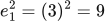
e_1=4-1=3Step 2: square error 1.
 LaTeX:
e_1^2=(3)^2=9Step 3: add squared errors.
 LaTeX:
\mathrm{SSE}=9=9Step 4: divide by 2 for half SSE.
 LaTeX:
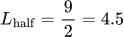
L_{\mathrm{half}}=\frac{9}{2}=4.5Step 5: divide by the number of predictions for MSE.
 LaTeX:
\mathrm{MSE}=\frac{9}{1}\approx9.000000000Final answer: SSE = 9; half SSE = 4.5; MSE ≈ 9.000000000.
Binary cross-entropy: target 1, predicted positive-class probability 0.8
Question. A binary classifier predicts P(y=1) = 0.8. The target is y = 1. Calculate binary cross-entropy using natural logarithms.
Given
Target y = 1; p = P(y=1) = 0.8; use natural log ln.
To find
The binary cross-entropy loss for this one example.
Formula — which one and why
The target selects the probability assigned to the correct class. Take its negative natural logarithm.
p is always the probability of class 1. When y = 0, the correct-class probability is 1−p.
 LaTeX:
L=-[y\ln p+(1-y)\ln(1-p)]Yaad rakhne ka cue: True class ki probability lo, uska minus ln lo.
Solution — step by step
Step 1: identify the correct-class probability.
 LaTeX:
p=0.8Step 2: evaluate its natural logarithm.
LaTeX: \ln(0.8)\approx-0.223143551Step 3: apply the minus sign outside the logarithm.
 LaTeX:
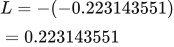
L=-(-0.223143551)=0.223143551Final answer: Loss ≈ 0.223143551 nats.
Binary cross-entropy: target 0, predicted positive-class probability 0.8
Question. A binary classifier predicts P(y=1) = 0.8. The target is y = 0. Calculate binary cross-entropy using natural logarithms.
Given
Target y = 0; p = P(y=1) = 0.8; use natural log ln.
To find
The binary cross-entropy loss for this one example.
Formula — which one and why
The target selects the probability assigned to the correct class. Take its negative natural logarithm.
p is always the probability of class 1. When y = 0, the correct-class probability is 1−p.
LaTeX: L=-[y\ln p+(1-y)\ln(1-p)]Yaad rakhne ka cue: True class ki probability lo, uska minus ln lo.
Solution — step by step
Step 1: identify the correct-class probability.
 LaTeX:
1-p=1-0.8=0.2Step 2: evaluate its natural logarithm.
 LaTeX:
\ln(0.2)\approx-1.609437912Step 3: apply the minus sign outside the logarithm.
 LaTeX:
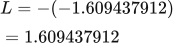
L=-(-1.609437912)=1.609437912Final answer: Loss ≈ 1.609437912 nats.
Binary cross-entropy: target 1, predicted positive-class probability 0.5
Question. A binary classifier predicts P(y=1) = 0.5. The target is y = 1. Calculate binary cross-entropy using natural logarithms.
Given
Target y = 1; p = P(y=1) = 0.5; use natural log ln.
To find
The binary cross-entropy loss for this one example.
Formula — which one and why
The target selects the probability assigned to the correct class. Take its negative natural logarithm.
p is always the probability of class 1. When y = 0, the correct-class probability is 1−p.
LaTeX: L=-[y\ln p+(1-y)\ln(1-p)]Yaad rakhne ka cue: True class ki probability lo, uska minus ln lo.
Solution — step by step
Step 1: identify the correct-class probability.
 LaTeX:
p=0.5Step 2: evaluate its natural logarithm.
 LaTeX:
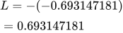
\ln(0.5)\approx-0.693147181Step 3: apply the minus sign outside the logarithm.
 LaTeX:
L=-(-0.693147181)=0.693147181Final answer: Loss ≈ 0.693147181 nats.
Sigmoid+BCE logit gradient: p=0.8, y=1
Question. A sigmoid output is p = 0.8 and target y = 1. For binary cross-entropy on one example, find the derivative with respect to the pre-sigmoid score z.
Given
p = 0.8; y = 1; single-example BCE; p = sigmoid(z).
To find
dL/dz, not dL/dp.
Formula — which one and why
Apply the chain rule to BCE followed backward through sigmoid. The factors p(1−p) cancel, leaving p−y.
p is an activated probability; z is its raw score; the requested derivative is with respect to z.
 LaTeX:
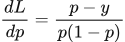
\frac{dL}{dp}=\frac{p-y}{p(1-p)}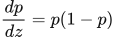 LaTeX:
\frac{dp}{dz}=p(1-p) LaTeX:
\frac{dL}{dz}=p-yYaad rakhne ka cue: BCE + sigmoid together ka shortcut p−y; chain already included.
Solution — step by step
Step 1: calculate the sigmoid slope.
 LaTeX:
p(1-p)=0.8(0.2)=0.16Step 2: differentiate BCE with respect to p.
 LaTeX:
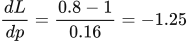
\frac{dL}{dp}=\frac{0.8-1}{0.16}=-1.25Step 3: multiply the two local derivatives.
 LaTeX:
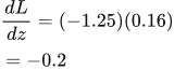
\frac{dL}{dz}=(-1.25)(0.16)=-0.2Final answer: dL/dz = -0.2. No further sigmoid derivative is needed.
Sigmoid+BCE logit gradient: p=0.8, y=0
Question. A sigmoid output is p = 0.8 and target y = 0. For binary cross-entropy on one example, find the derivative with respect to the pre-sigmoid score z.
Given
p = 0.8; y = 0; single-example BCE; p = sigmoid(z).
To find
dL/dz, not dL/dp.
Formula — which one and why
Apply the chain rule to BCE followed backward through sigmoid. The factors p(1−p) cancel, leaving p−y.
p is an activated probability; z is its raw score; the requested derivative is with respect to z.
LaTeX: \frac{dL}{dp}=\frac{p-y}{p(1-p)}LaTeX: \frac{dp}{dz}=p(1-p)LaTeX: \frac{dL}{dz}=p-yYaad rakhne ka cue: BCE + sigmoid together ka shortcut p−y; chain already included.
Solution — step by step
Step 1: calculate the sigmoid slope.
LaTeX: p(1-p)=0.8(0.2)=0.16Step 2: differentiate BCE with respect to p.
 LaTeX:
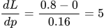
\frac{dL}{dp}=\frac{0.8-0}{0.16}=5Step 3: multiply the two local derivatives.
 LaTeX:
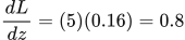
\frac{dL}{dz}=(5)(0.16)=0.8Final answer: dL/dz = 0.8. No further sigmoid derivative is needed.