Deep Learning · MT2 · section
AdaGrad adds every squared gradient
Optimization algorithms
Definition. AdaGrad is an adaptive first-order optimizer that scales each parameter's update using the inverse square root of the sum of its previous and current squared gradients. Each parameter maintains its own accumulator.
State, effective learning rate and update
For one parameter θ, let gₜ be its current gradient and s₀ = 0:
 LaTeX:
s_t=s_{t-1}+g_t^2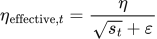 LaTeX:
\eta_{\mathrm{effective},t}=\frac{\eta}{\sqrt{s_t}+\varepsilon} LaTeX:
\theta_t=\theta_{t-1}-\eta_{\mathrm{effective},t}g_ts stores squared-gradient history. Both positive and negative gradients increase this nonnegative sum after squaring. The effective learning rate is the coefficient multiplying the signed gradient; the actual displacement also depends on that gradient's magnitude and sign.
Complete numerical: supplied gradients
Question. Start θ₀ = 1, s₀ = 0, η = 0.1. Given gradients g₁ = 2 and g₂ = 1, perform two AdaGrad updates. Ignore epsilon only for this hand calculation because neither denominator is zero.
Given
θ₀ = 1; initial state(s) = 0; η = 0.1.
Supplied gradients g₁ = 2, g₂ = 1.
ε = 0 for this hand calculation.
To find
Calculate all required states and the parameter after each of two updates.
Formula — which one and why
AdaGrad. Add the new squared gradient to all previous squares. Divide the signed current gradient by the square root of that accumulated magnitude.
G = accumulated squared gradients (also denoted s in some lessons); g = current gradient; η = base learning rate; ε = small stabilizer, set to zero only where the question says so.
 LaTeX:
G_t=G_{t-1}+g_t^2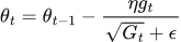 LaTeX:
\theta_t=\theta_{t-1}-\frac{\eta g_t}{\sqrt{G_t}+\epsilon}Yaad rakhne ka cue: Square karo, purane sum mein jodo, root se scale karo.
Solution — step by step
The gradients are supplied by the question. They are not computed from an assumed objective, and g₂ is not replaced by the updated parameter.
Iteration 1 — step 1: update the accumulator.
 LaTeX:
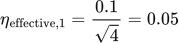
s_1=0+2^2=4Step 2: calculate the effective learning rate.
 LaTeX:
\eta_{\mathrm{effective},1}=\frac{0.1}{\sqrt4}=0.05Step 3: apply the signed gradient.
 LaTeX:
\theta_1=1-0.05(2)=0.9Iteration 2 — step 1: retain s₁ and add the new squared gradient.
 LaTeX:
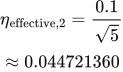
s_2=4+1^2=5Step 2: calculate the new coefficient.
 LaTeX:
\eta_{\mathrm{effective},2}=\frac{0.1}{\sqrt5}\approx0.044721360Step 3: update from θ₁.
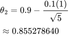 LaTeX:
\theta_2=0.9-\frac{0.1(1)}{\sqrt5}\approx0.855278640Final answer: θ₁ = 0.9 and θ₂ ≈ 0.855279, with accumulators s₁ = 4 and s₂ = 5.
Advantage, limitation and epsilon convention
Coordinate-specific scaling can be useful when some features or gradients occur infrequently. Because s never decreases, its effective learning rate is nonincreasing when η and ε are fixed, and can become too small during prolonged training. The actual displacement magnitude need not decrease monotonically because gₜ also changes.
ε is normally a small positive stabilizer. These notes place it outside the square root. If a question places it inside, use that specified denominator consistently; the two placements are not numerically identical.