Deep Learning · MT2 · section

Adam bias correction: why the denominator is one minus beta to a power

Optimization algorithms

Definition. Bias correction compensates for the reduced total observation weight caused by initializing an exponentially weighted accumulator to zero. Under a stationary gradient expectation, it removes the corresponding initialization bias in the moment estimate.

Explanation and working

1. What the moving average actually contains

Adam's signed-gradient memory is m. Starting with m₀ = 0 and β = 0.9, the first average is 90% of zero plus 10% of the first gradient. If g₁ = 2, then m₁ = 0.2. That small value partly reflects the artificial zero initialization.

Diagram: The first raw average is pulled toward its starting zero. Divide by the missing-weight correction factor.. Labels: Correct the early zero-initialized memory | Correct the early zero-initialized memory | Example: β₁ = 0.9, first gradient = 2, initial m = 0. | Raw memory | m₁ = 0.9 × 0 + 0.1 × | 2 = 0.2 | Correction factor | 1 − 0.9¹ = 0.1 | Corrected memory | m̂₁ = 0.2 ÷ 0.1 = 2 | The small raw value is partly caused by the starting zero. Bias correction | removes that effect.

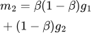
LaTeX: m_1=(1-\beta)g_1

At the second step, substitute the first expression into the recurrence:

LaTeX: m_2=\beta(1-\beta)g_1+(1-\beta)g_2

2. Add the coefficients

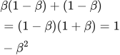
After the first step, the total coefficient attached to observed gradients is 1 − β. After two steps it is β(1 − β) + (1 − β). Factor out the common term:

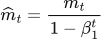
LaTeX: \beta(1-\beta)+(1-\beta)=(1-\beta)(1+\beta)=1-\beta^2

After t steps the coefficients sum to 1 − βᵗ. Dividing the stored average by that quantity removes this zero-start coefficient deficit.

LaTeX: \widehat m_t=\frac{m_t}{1-\beta_1^t}

The squared-gradient memory uses its own decay β₂ and the same reasoning:

LaTeX: \widehat s_t=\frac{s_t}{1-\beta_2^t}

3. A constant-gradient example makes the purpose visible

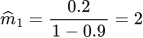
Let both gradients be 2 and use β₁ = 0.9. The first raw mean is 0.2; the second is 0.9 × 0.2 + 0.1 × 2 = 0.38.

LaTeX: \widehat m_1=\frac{0.2}{1-0.9}=2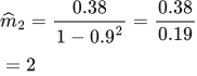

LaTeX: \widehat m_2=\frac{0.38}{1-0.9^2}=\frac{0.38}{0.19}=2

Both corrected values now equal the constant observed gradient. If gradients differ over time, the corrected result is a weighted average, not necessarily the latest gradient.

4. Two betas mean two separate powers

At update 2 with β₁ = 0.9 and β₂ = 0.999, the first correction denominator is 1 − 0.9² = 0.19. The second is 1 − 0.999² = 0.001999. Do not use 0.19 for both memories, and do not keep using the first-step denominators.

5. Correct first, then combine

The parameter update uses the corrected signed mean divided by the square root of the corrected squared mean, plus ε in the stated position. The square root is taken after correcting s. The numerator is not the loss, and no extra multiplication by g follows.

This derivation explains the formula; the following solved Adam examples show the complete arithmetic when gradients change sign or magnitude.