Deep Learning · MT2 · section

A moving average remembers the recent past

Optimization algorithms

Definition. An exponentially weighted moving average (EWMA) is a recursively updated estimate in which older observations receive exponentially decreasing weights. Optimizers use it to summarize recent gradients or squared gradients.

For m₀ = 0, expanding the recurrence gives:

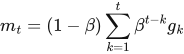
$m_t=(1-\beta)\sum_{k=1}^{t}\beta^{t-k}g_k$ LaTeX: m_t=(1-\beta)\sum_{k=1}^{t}\beta^{t-k}g_k

The most recent gradient has coefficient 1 − β; a gradient k steps older is discounted by an additional factor βᵏ. Larger β smooths more strongly but responds more slowly to a change in direction. The heuristic averaging horizon is approximately 1/(1 − β); it is not a hard cutoff in the stored history.

Signed gradients versus squared gradients

An average of g contains directional information: positive and negative contributions can cancel. An average of g² estimates the scale through an uncentered second moment and cannot become negative when initialized nonnegatively. Adam tracks both quantities. RMSProp tracks a squared-gradient average in its basic form.

Question. Let β = 0.9, m₀ = 0 and gradients g₁ = 2, g₂ = −1. Find m₁ and m₂.

Given

β = 0.9; initial m₀ = 0.

Gradients in order: g₁ = 2, g₂ = −1.

To find

Find m₁ and m₂, preserving the sign of each gradient.

Formula — which one and why

Exponential moving average. Keep the specified fraction of the old state and add the complementary fraction of the new gradient. This tracks signed direction, so negative gradients can reduce the state.

β (beta) = retained fraction; m = stored average; g = current gradient. m₀ is the initial state.

$m_t=\beta m_{t-1}+(1-\beta)g_t$ LaTeX: m_t=\beta m_{t-1}+(1-\beta)g_t

Yaad rakhne ka cue: Beta purani memory rakhta hai; 1−beta naya gradient leta hai.

Solution — step by step

Step 1: find the recent-gradient coefficient.

$1-0.9=0.1$ LaTeX: 1-0.9=0.1

Step 2: retain the old memory for step 1.

$0.9(0)=0$ LaTeX: 0.9(0)=0

Step 3: weight the first gradient.

$0.1(2)=0.2$ LaTeX: 0.1(2)=0.2

Step 4: add to obtain the first memory.

$m_1=0+0.2=0.2$ LaTeX: m_1=0+0.2=0.2

Step 5: retain the first memory for step 2.

$0.9(0.2)=0.18$ LaTeX: 0.9(0.2)=0.18

Step 6: weight the second gradient.

$0.1(-1)=-0.1$ LaTeX: 0.1(-1)=-0.1

Step 7: add to obtain the second memory.

$m_2=0.18+(-0.1)=0.08$ LaTeX: m_2=0.18+(-0.1)=0.08

Final answer: m₁ = 0.2; m₂ = 0.08.

The second average remains positive although the latest gradient is negative because the previous positive contribution still has weight. If the recurrence is applied to the squared gradients instead, the second state is 0.9(0.4) + 0.1(1) = 0.46. These states have different meanings and are not interchangeable.