Deep Learning · MT2 · section
L1 and L2 add a cost for large weights
Regularization and generalization
Definition. Regularization modifies a training objective or learning procedure to constrain the fitted model and improve generalization. L1 and L2 regularization add parameter-norm penalties to the data loss.
Explanation and working
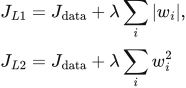 LaTeX:
J_{L1}=J_{\mathrm{data}}+\lambda\sum_i|w_i|,\qquad J_{L2}=J_{\mathrm{data}}+\lambda\sum_iw_i^2Lambda controls how strongly you discourage weight size. L1 encourages sparsity, meaning many weights can become exactly zero under suitable optimization. L2 shrinks weights smoothly and usually leaves small nonzero values. Larger lambda can reduce overfitting, but excessive regularization can underfit.
Question. Data loss = 0.5; weights [2, −1]; λ = 0.1. Compute L1-regularized and L2-regularized objectives using the displayed convention.
Given
Data loss = 0.5; weights = [2,−1]; λ = 0.1.
The L2 convention here has no factor ½.
To find
Find L1/L2 penalties and the two regularized objective values.
Formula — which one and why
L1 penalty and gradient. Add absolute weight magnitudes to penalize large weights. Away from zero, the penalty derivative depends on the weight’s sign.
λ (lambda) = penalty strength; J_data = data loss; sign(w) is +1 for positive and −1 for negative weights. At zero a subgradient convention is needed.
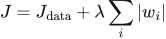 LaTeX:
J=J_{\mathrm{data}}+\lambda\sum_i|w_i| LaTeX:
g_i=g_{\mathrm{data},i}+\lambda\operatorname{sign}(w_i)Yaad rakhne ka cue: L1 absolute values leta hai; gradient mein sign aata hai.
L2 penalty without a factor of one-half. This stated convention multiplies the sum of squares by λ, so differentiating contributes 2λw. Do not use the half-scaled gradient for this objective.
λ = penalty strength; J_data = original data loss; wᵢ = weight i.
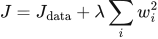 LaTeX:
J=J_{\mathrm{data}}+\lambda\sum_iw_i^2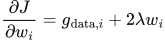 LaTeX:
\frac{\partial J}{\partial w_i}=g_{\mathrm{data},i}+2\lambda w_iYaad rakhne ka cue: Half nahi diya toh L2 derivative mein 2 lambda × weight.
Solution — step by step
Step 1: take absolute values for L1.
 LaTeX:
|2|=2,\qquad|-1|=1Step 2: add the absolute values.
 LaTeX:
2+1=3Step 3: multiply by lambda.
 LaTeX:
0.1(3)=0.3Step 4: add the data loss.
 LaTeX:
J_{L1}=0.5+0.3=0.8Step 5: square both weights for L2.
 LaTeX:
2^2=4,\qquad(-1)^2=1Step 6: add the squares.
 LaTeX:
4+1=5Step 7: multiply by lambda without adding a half.
 LaTeX:
0.1(5)=0.5Step 8: add the data loss.
 LaTeX:
J_{L2}=0.5+0.5=1.0For this L2 convention, the additional gradient is 2 λw. If the objective uses λ/2 times the squared sum, the additional gradient is λw instead. The factor is decided by the stated objective.
L2 gradient update without a half factor
Question. A weight is 2, its data-loss gradient is 0.3, λ = 0.1 and η = 0.01. The objective adds λw². Perform one update.
Given
w = 2; data gradient = 0.3; λ = 0.1; η = 0.01. The penalty has no factor ½.
To find
Penalty gradient, total gradient and updated weight.
Formula — which one and why
The derivative of λw² is 2λw. Add it to the data gradient before applying gradient descent.
λ is penalty strength; η is learning rate; g is the full objective gradient.
 LaTeX:
g_{\mathrm{penalty}}=2\lambda w LaTeX:
g=g_{\mathrm{data}}+g_{\mathrm{penalty}} LaTeX:
w_{\mathrm{new}}=w-\eta gYaad rakhne ka cue: Penalty ka gradient data gradient mein jodo, phir update.
Solution — step by step
Step 1: calculate the penalty gradient.
 LaTeX:
2(0.1)(2)=0.4Step 2: add the data gradient.
 LaTeX:
g=0.3+0.4=0.7Step 3: scale by the learning rate.
 LaTeX:
\eta g=0.01(0.7)=0.007Step 4: subtract from the old weight.
 LaTeX:
w_{\mathrm{new}}=2-0.007=1.993Final answer: Updated weight = 1.993. Bias penalties are omitted unless the objective includes them.
Deriving the L2 update
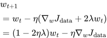
Under the objective written above, the data gradient and penalty gradient add:
 LaTeX:
\nabla_w J=\nabla_w J_{\mathrm{data}}+2\lambda wFor ordinary gradient descent, regrouping the update gives:
 LaTeX:
w_{t+1}=w_t-\eta(\nabla_w J_{\mathrm{data}}+2\lambda w_t)=(1-2\eta\lambda)w_t-\eta\nabla_w J_{\mathrm{data}}This shows the shrinkage associated with this L2 convention. For an objective containing λ‖w‖²/2, replace 2λ by λ. This algebra explains the equivalence to appropriately scaled weight decay for ordinary gradient descent; adding an L2 term inside an adaptive optimizer is generally different from decoupled weight decay.