Deep Learning · MT2 · section
Applications of convolutional neural networks
CNN architectures and transfer learning
Definition. A CNN application combines a convolutional feature extractor with an output head designed for a particular prediction task. Shared local filters learn spatial patterns; the output head determines what is predicted and the loss determines how it is trained.
Classification, detection and segmentation
| Task | Required output | What distinguishes it |
|---|---|---|
| Image classification | One label or class distribution for the image | Answers what category the whole image belongs to |
| Object detection | Object classes and bounding-box coordinates | Also identifies where each detected object is located |
| Semantic segmentation | A class label or distribution for each pixel | Produces a spatial label map rather than one image-wide class |
| Face recognition | Identity class or a learned face representation | Compares or classifies learned visual features |
A softmax image classifier alone does not produce boxes or pixel labels. Detection and segmentation require appropriate task heads, targets and objectives. In an applications question, explain the prediction required instead of listing model names without their purpose.
Examples across domains
Medical imaging: classify an image or use a segmentation model to identify regions of interest. The target may be an image-level label or a pixel mask, so the architecture and loss must match that choice.
Autonomous perception: use camera images for tasks such as detecting pedestrians and vehicles or segmenting road regions. These outputs are inputs to a larger perception and decision system.
Manufacturing: classify product images as defective or non-defective, or localize defects when position information is needed.
Document analysis: classify cropped handwritten characters; a complete document-reading system must also locate and order text regions.
Remote sensing: classify land-use regions or segment different surface categories in satellite images. Spatial context and texture can help distinguish classes.
Complete exam-style application answer
Question. Describe how a CNN can classify product photographs into three classes: acceptable, scratched and cracked. Explain the input, network stages, output activation, loss, training and evaluation.
Step 1: define data and labels. Each example contains an image and one of the three class labels. Use separate training, validation and test sets, keeping near-duplicate photographs of the same item out of different splits. Apply the chosen model's input size and scaling consistently.
Step 2: extract spatial features. Convolutional layers calculate local responses using shared kernels. Nonlinear activations allow more complex combinations of those responses. Further convolution stages combine local patterns; pooling may reduce spatial dimensions.
Step 3: produce three class scores. Convert the final representation into a feature vector, using flattening or an appropriate global pooling operation, and apply a dense layer with three outputs. These raw outputs are logits.
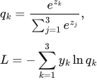
Step 4: calculate class probabilities and loss. For mutually exclusive classes, use softmax and categorical cross-entropy. A one-hot label selects the probability of the correct class.
 LaTeX:
q_k=\frac{e^{z_k}}{\sum_{j=1}^{3}e^{z_j}},\qquad L=-\sum_{k=1}^{3}y_k\ln q_kStep 5: train the parameters. Run forward propagation, evaluate the loss, backpropagate derivatives and update the trainable convolutional and dense parameters using the selected optimizer. Use validation results for hyperparameters and stopping decisions.
Step 6: evaluate the selected model. Assess the final model on held-out photographs. Report overall classification performance and inspect which defects are confused. With limited data, a pretrained CNN can provide features and selected layers can be fine-tuned.
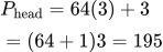
Numerical extension. If the last pooled feature vector has 64 components, how many parameters does the three-class dense head have, including bias?
Step 1: each output receives 64 weights, so three outputs require 64 × 3 = 192 weights.
Step 2: each of the three outputs has one bias, giving 3 biases.
 LaTeX:
P_{\mathrm{head}}=64(3)+3=(64+1)3=195Final answer: 195 trainable parameters in this head. Softmax adds no trainable parameters. The backbone's parameters are counted separately.