Deep Learning · TEE · formulas
Gradient descent
A gradient tells us the local direction in which loss rises. Gradient descent subtracts a small multiple of that gradient. Learning rate η controls the size of this correction. After the first update, calculate the next gradient at the new parameter.
 LaTeX:
\theta_{new}=\theta-\eta g LaTeX:
g=\frac{\partial J}{\partial\theta}Reading an optimizer formula without getting lost
An optimizer updates the numbers the model is allowed to learn. Usually these are weights and biases. The letter θ is a convenient name for whichever parameter is currently being updated.
Old, current and new
At update t, θₜ₋₁ is the value before the update and θₜ is the value after it. The symbol gₜ is the loss gradient used in that update. If a question already supplies gₜ, use it. If it supplies a loss J(θ), differentiate J and evaluate the derivative at the stated position.
 LaTeX:
\theta_t=\theta_{t-1}-\eta g_tη, read eta, is the learning rate. It multiplies the gradient to determine the basic correction. A positive gradient is subtracted; a negative gradient makes the new value larger because subtracting a negative is addition.
What a stored state means
An optimizer may retain a number from its previous update. This number is called its state or memory. It is an ordinary calculated number, not an additional neuron. Momentum stores movement; AdaGrad stores a sum of squared gradients; RMSProp stores a moving average of squares; Adam stores a moving average of gradients and another of squares.
A weighted average from ordinary arithmetic
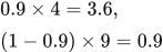
If the old state is 4, the new squared gradient is 9 and the decay is 0.9, retain 90% of the old state and add 10% of the new square.
 LaTeX:
0.9\times4=3.6,\qquad(1-0.9)\times9=0.9 LaTeX:
s_{\mathrm{new}}=3.6+0.9=4.5The coefficients 0.9 and 0.1 add to 1. As updates continue, a past contribution gets multiplied by 0.9 again, so its influence fades. AdaGrad instead gives 4 + 9 = 13 because it retains the full old sum.
Squared memory and signed direction
For gradient −3, the square is 9. The stored scale is positive, but the update still needs the negative gradient to determine direction. Do not replace every occurrence of g with g².
Epsilon and hats
ε, read epsilon, is a small positive number that prevents an exactly zero denominator. A hat in Adam, such as m with a hat, labels a bias-corrected average. A hat does not mean squaring. The power βᵗ uses the update number t, so its value changes from the first update to the second.
The ordinary gradient descent update
Definition. Gradient descent is an iterative first-order optimization algorithm that updates parameters in the negative direction of the current objective gradient, scaled by a positive learning rate.
Explanation and working
 LaTeX:
g_t=J\prime(\theta_{t-1})LaTeX: \theta_t=\theta_{t-1}-\eta g_tHere update numbers start at t = 1: calculate g₁ at θ₀, obtain θ₁, then calculate g₂ at θ₁. The subscript counts completed updates; it is not an exponent.
Read it aloud: “new parameter equals old parameter minus learning rate times current gradient.” The old parameter is where you are. The gradient gives the local uphill direction. The learning rate controls how far you move in the opposite direction.
Question. J(θ) = 0.7 θ³; θ₀ = 1; η = 0.1. Perform two iterations.
Given
J(θ) = 0.7θ³; initial θ₀ = 1; η = 0.1.
To find
Differentiate J and perform two gradient-descent iterations.
Formula — which one and why
Gradient descent. Evaluate the gradient at the current parameter, multiply by the learning rate and subtract. If the objective is supplied, differentiate it and recompute the gradient after each update.
θ (theta) = trainable parameter; g = derivative of the stated objective J; η = learning rate; t labels the update number.
LaTeX: g_t=J\prime(\theta_{t-1})LaTeX: \theta_t=\theta_{t-1}-\eta g_tYaad rakhne ka cue: Naya = purana − learning rate × current gradient.
Solution — step by step
Step 1. Differentiate. g(θ) = 0.7 × 3 × θ² = 2.1 θ².
Step 2. First update. g₁ = 2.1(1)² = 2.1. θ₁ = 1 − 0.1(2.1) = 0.79.
Step 3. Second gradient. Square the new value: 0.79² = 0.6241. Multiply: g₂ = 2.1 × 0.6241 = 1.31061.
Step 4. Second update. θ₂ = 0.79 − 0.1(1.31061) = 0.79 − 0.131061 = 0.658939.
The paper calls this SGD. With only a scalar objective supplied, no sample selection is specified; the arithmetic is the stated gradient-descent update. Also, this cubic is not bounded below over all real values. Do not claim these two steps prove convergence to a global minimum.
Common error: using the loss J itself instead of its derivative g. Another error is repeatedly using θ₀ to calculate later gradients.
Drill 18 GD variation 1
Question
Question. J(θ) = ½θ², θ₀ = 1, η = 0.1. Perform two GD updates.
Answer — step by step
Given
Objective: J(θ) = ½θ².
Initial θ₀ = 1; η = 0.1; two iterations.
To find
Find every stored state needed by the method and the parameter after each of two updates.
Formula — which one and why
Gradient descent. Evaluate the gradient at the current parameter, multiply by the learning rate and subtract. If the objective is supplied, differentiate it and recompute the gradient after each update.
θ (theta) = trainable parameter; g = derivative of the stated objective J; η = learning rate; t labels the update number.
LaTeX: g_t=J\prime(\theta_{t-1})LaTeX: \theta_t=\theta_{t-1}-\eta g_tYaad rakhne ka cue: Naya = purana − learning rate × current gradient.
Solution — step by step
Meaning of the symbols
θ (theta) is the number we update. η (eta) is learning rate 0.1. g is the derivative of the objective, evaluated at the required position. A subscript counts updates; θ₀ means the starting value.
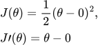
Differentiate the objective first
 LaTeX:
J(\theta)=\frac12(\theta-0)^2,\qquad J\prime(\theta)=\theta-0The power rule brings down 2, which cancels the half. The inside derivative is 1, so the remaining gradient is θ minus 0.
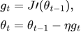
Update formulas
 LaTeX:
g_t=J\prime(\theta_{t-1}),\quad \theta_t=\theta_{t-1}-\eta g_tStep 1: Update 1.
 LaTeX:
g_1=1-(0)=1 LaTeX:
\theta_1=1-0.1(1)=0.9Step 2: Update 2.
 LaTeX:
g_2=0.9-(0)=0.9 LaTeX:
\theta_2=0.9-0.1(0.9)=0.81Final parameter after two updates: 0.81. The second gradient is evaluated again using the parameter obtained after the first update.
Drill 19 GD variation 2
Question
Question. J(θ) = ½(θ−1)², θ₀ = -0.5, η = 0.1. Perform two GD updates.
Answer — step by step
Given
Objective: J(θ) = ½(θ−1)².
Initial θ₀ = −0.5; η = 0.1; two iterations.
To find
Find every stored state needed by the method and the parameter after each of two updates.
Formula — which one and why
Gradient descent. Evaluate the gradient at the current parameter, multiply by the learning rate and subtract. If the objective is supplied, differentiate it and recompute the gradient after each update.
θ (theta) = trainable parameter; g = derivative of the stated objective J; η = learning rate; t labels the update number.
LaTeX: g_t=J\prime(\theta_{t-1})LaTeX: \theta_t=\theta_{t-1}-\eta g_tYaad rakhne ka cue: Naya = purana − learning rate × current gradient.
Solution — step by step
Meaning of the symbols
θ (theta) is the number we update. η (eta) is learning rate 0.1. g is the derivative of the objective, evaluated at the required position. A subscript counts updates; θ₀ means the starting value.
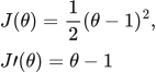
Differentiate the objective first
 LaTeX:
J(\theta)=\frac12(\theta-1)^2,\qquad J\prime(\theta)=\theta-1The power rule brings down 2, which cancels the half. The inside derivative is 1, so the remaining gradient is θ minus 1.
Update formulas
LaTeX: g_t=J\prime(\theta_{t-1}),\quad \theta_t=\theta_{t-1}-\eta g_tStep 1: Update 1.
 LaTeX:
g_1=-0.5-(1)=-1.5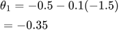 LaTeX:
\theta_1=-0.5-0.1(-1.5)=-0.35Step 2: Update 2.
 LaTeX:
g_2=-0.35-(1)=-1.35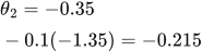 LaTeX:
\theta_2=-0.35-0.1(-1.35)=-0.215Final parameter after two updates: -0.215. The second gradient is evaluated again using the parameter obtained after the first update.
Drill 6 Chain rule on a tiny loss
Question
Question. Let o = wx+b, L = ½(o−y)², x = 3, w = 0.2, b = 0.1, y = 1. Find dL/dw, dL/db and update at η = 0.1.
Answer — step by step
Given
Model: o = wx+b; loss L = ½(o−y)².
x = 3; y = 1; w = 0.2; b = 0.1.
Learning rate η = 0.1.
To find
Find ∂L/∂w, ∂L/∂b and the updated weight and bias.
Formula — which one and why
Chain rule for a linear neuron. The weight changes the prediction, and the prediction changes the loss. Multiply those two local rates. Half squared loss differentiates to prediction minus target; the neuron contributes input x.
z = prediction; y = target; e = z−y; g_w and g_b = loss derivatives for weight and bias. ∂L/∂w means “how fast loss changes when w changes”. η (eta) = learning rate.
 LaTeX:
z=wx+b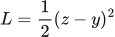 LaTeX:
L=\frac12(z-y)^2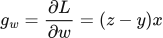 LaTeX:
g_w=\frac{\partial L}{\partial w}=(z-y)x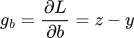 LaTeX:
g_b=\frac{\partial L}{\partial b}=z-y LaTeX:
w_{\mathrm{new}}=w-\eta g_w LaTeX:
b_{\mathrm{new}}=b-\eta g_bYaad rakhne ka cue: Ek path mein multiply; alag paths mil rahe hon toh add.
Solution — step by step
Meaning and formulas
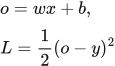
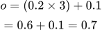
The output o is a linear prediction: no sigmoid or ReLU is specified. Changing w changes o, which changes L. The chain rule multiplies those linked effects.
 LaTeX:
o=wx+b,\qquad L=\frac12(o-y)^2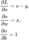 LaTeX:
\frac{\partial L}{\partial o}=o-y,\quad \frac{\partial o}{\partial w}=x,\quad \frac{\partial o}{\partial b}=1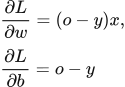 LaTeX:
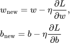
\frac{\partial L}{\partial w}=(o-y)x,\qquad \frac{\partial L}{\partial b}=o-yThe learning rate η says how much of the gradient to subtract.
 LaTeX:
w_{\mathrm{new}}=w-\eta\frac{\partial L}{\partial w},\qquad b_{\mathrm{new}}=b-\eta\frac{\partial L}{\partial b}Step 1: obtain the current prediction and error
 LaTeX:
o=(0.2\times3)+0.1=0.6+0.1=0.7 LaTeX:
o-y=0.7-1=-0.3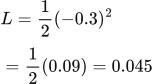 LaTeX:
L=\frac12(-0.3)^2=\frac12(0.09)=0.045Step 2: calculate both gradients from this same prediction
 LaTeX:
\frac{\partial L}{\partial w}=(-0.3)\times3=-0.9 LaTeX:
\frac{\partial L}{\partial b}=(-0.3)\times1=-0.3Step 3: update the weight
 LaTeX:
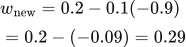
w_{\mathrm{new}}=0.2-0.1(-0.9)=0.2-(-0.09)=0.29Step 4: update the bias
 LaTeX:
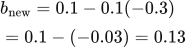
b_{\mathrm{new}}=0.1-0.1(-0.3)=0.1-(-0.03)=0.13Final answer: weight gradient −0.9; bias gradient −0.3; new weight 0.29; new bias 0.13. Both updates use the old forward pass.