Deep Learning · TEE · formulas
Nesterov: look-ahead gradient
Nesterov first uses the old movement to choose a temporary look-ahead position. It measures the gradient there, calculates the new movement, then adds that movement to the original parameter. The temporary look-ahead position does not replace the original parameter in the final addition.
 LaTeX:
\theta_{look}=\theta+\beta v LaTeX:
v_{new}=\beta v-\eta g(\theta_{look}) LaTeX:
\theta_{new}=\theta+v_{new}Nesterov looks before correcting
Definition. Nesterov accelerated gradient is a momentum-based method that evaluates the gradient at a lookahead parameter, formed using the previous velocity, before calculating the new velocity and actual parameter update.
What changes relative to momentum
Ordinary momentum evaluates J′ at θₜ₋₁. Nesterov evaluates it after the anticipated displacement βvₜ₋₁. This changes the point where the objective's slope is measured:
 LaTeX:
\theta_{\mathrm{look},t}=\theta_{t-1}+\beta v_{t-1} LaTeX:
g_t=J'(\theta_{\mathrm{look},t}) LaTeX:
v_t=\beta v_{t-1}-\eta g_t LaTeX:
\theta_t=\theta_{t-1}+v_tThe lookahead point is an auxiliary evaluation point, not the new actual parameter. In this signed-displacement convention, the new velocity is added to θₜ₋₁.
Complete numerical: two iterations
Question. J(θ) = ½θ², θ₀ = 1, v₀ = 0, η = 0.1 and β = 0.9. Perform two Nesterov updates using signed displacement velocity.
Given
J(θ) = ½θ²; θ₀ = 1; v₀ = 0.
η = 0.1; β = 0.9; signed-displacement velocity.
To find
Find the gradient, velocity and actual parameter after each of two iterations.
Formula — which one and why
Nesterov lookahead. First look ahead using the old velocity. Measure the gradient there, form the new velocity, then add that velocity to the original current parameter.
θ_look = temporary gradient-evaluation point; v = signed displacement; β = momentum coefficient; η = learning rate.
 LaTeX:
\theta_{\mathrm{look}}=\theta_{t-1}+\beta v_{t-1} LaTeX:
g_t=J\prime(\theta_{\mathrm{look}})LaTeX: v_t=\beta v_{t-1}-\eta g_tLaTeX: \theta_t=\theta_{t-1}+v_tYaad rakhne ka cue: Pehle look ahead; gradient wahan; update original position se.
Solution — step by step
The derivative is J′(θ) = θ. Therefore the gradient equals the lookahead value in this particular objective.
Iteration 1 — step 1: locate the lookahead point.
 LaTeX:
\theta_{\mathrm{look},1}=1+0.9(0)=1Step 2: evaluate the gradient there.
 LaTeX:
g_1=J'(1)=1Step 3: calculate the new velocity and actual parameter.
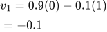 LaTeX:
v_1=0.9(0)-0.1(1)=-0.1 LaTeX:
\theta_1=1+(-0.1)=0.9Iteration 2 — step 1: use the previous actual parameter and velocity.
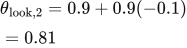 LaTeX:
\theta_{\mathrm{look},2}=0.9+0.9(-0.1)=0.81Step 2: evaluate the gradient at 0.81, not at 0.9.
 LaTeX:
g_2=J'(0.81)=0.81Step 3: calculate the new velocity.
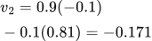 LaTeX:
v_2=0.9(-0.1)-0.1(0.81)=-0.171Step 4: update the old actual parameter.
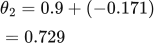 LaTeX:
\theta_2=0.9+(-0.171)=0.729| Iteration | Old actual θ | Lookahead θ | Gradient | New v | New actual θ |
|---|---|---|---|---|---|
| 1 | 1 | 1 | 1 | −0.1 | 0.9 |
| 2 | 0.9 | 0.81 | 0.81 | −0.171 | 0.729 |
Final answer: θ₁ = 0.9 and θ₂ = 0.729. The first update matches ordinary momentum because v₀ = 0. At the second update, ordinary momentum would use gradient 0.9 and produce θ₂ = 0.72. Adding v₂ to 0.81 instead of 0.9 would count the old momentum contribution twice.
Drill 22 Nesterov variation 1
Question
Question. J(θ) = ½θ², θ₀ = 1, η = 0.1. Perform two Nesterov updates. Use β = 0.9, v₀ = 0 and signed velocity.
Answer — step by step
Given
Objective: J(θ) = ½θ².
Initial θ₀ = 1; η = 0.1; two iterations.
β = 0.9; initial signed velocity v₀ = 0.
To find
Find every stored state needed by the method and the parameter after each of two updates.
Formula — which one and why
Nesterov lookahead. First look ahead using the old velocity. Measure the gradient there, form the new velocity, then add that velocity to the original current parameter.
θ_look = temporary gradient-evaluation point; v = signed displacement; β = momentum coefficient; η = learning rate.
LaTeX: \theta_{\mathrm{look}}=\theta_{t-1}+\beta v_{t-1}LaTeX: g_t=J\prime(\theta_{\mathrm{look}})LaTeX: v_t=\beta v_{t-1}-\eta g_tLaTeX: \theta_t=\theta_{t-1}+v_tYaad rakhne ka cue: Pehle look ahead; gradient wahan; update original position se.
Solution — step by step
Meaning of the symbols
θ (theta) is the number we update. η (eta) is learning rate 0.1. g is the derivative of the objective, evaluated at the required position. A subscript counts updates; θ₀ means the starting value.
Differentiate the objective first
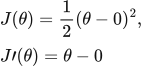 LaTeX:
J(\theta)=\frac12(\theta-0)^2,\qquad J\prime(\theta)=\theta-0The power rule brings down 2, which cancels the half. The inside derivative is 1, so the remaining gradient is θ minus 0.
Update formulas
v stores the signed movement from the previous update. β = 0.9 retains 90% of that movement. Start v₀ = 0.
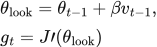 LaTeX:
\theta_{\mathrm{look}}=\theta_{t-1}+\beta v_{t-1},\quad g_t=J\prime(\theta_{\mathrm{look}})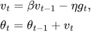 LaTeX:
v_t=\beta v_{t-1}-\eta g_t,\quad \theta_t=\theta_{t-1}+v_tStep 1: Update 1.
 LaTeX:
\theta_{\mathrm{look}}=1+0.9(0)=1 LaTeX:
g_1=1-(0)=1LaTeX: v_1=0.9(0)-0.1(1)=-0.1LaTeX: \theta_1=1+(-0.1)=0.9Step 2: Update 2.
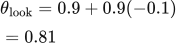 LaTeX:
\theta_{\mathrm{look}}=0.9+0.9(-0.1)=0.81 LaTeX:
g_2=0.81-(0)=0.81LaTeX: v_2=0.9(-0.1)-0.1(0.81)=-0.171LaTeX: \theta_2=0.9+(-0.171)=0.729Final parameter after two updates: 0.729. The lookahead locates the gradient; the new velocity is added to the old actual parameter, not to the lookahead.
Drill 23 Nesterov variation 2
Question
Question. J(θ) = ½(θ−1)², θ₀ = -0.5, η = 0.1. Perform two Nesterov updates. Use β = 0.9, v₀ = 0 and signed velocity.
Answer — step by step
Given
Objective: J(θ) = ½(θ−1)².
Initial θ₀ = −0.5; η = 0.1; two iterations.
β = 0.9; initial signed velocity v₀ = 0.
To find
Find every stored state needed by the method and the parameter after each of two updates.
Formula — which one and why
Nesterov lookahead. First look ahead using the old velocity. Measure the gradient there, form the new velocity, then add that velocity to the original current parameter.
θ_look = temporary gradient-evaluation point; v = signed displacement; β = momentum coefficient; η = learning rate.
LaTeX: \theta_{\mathrm{look}}=\theta_{t-1}+\beta v_{t-1}LaTeX: g_t=J\prime(\theta_{\mathrm{look}})LaTeX: v_t=\beta v_{t-1}-\eta g_tLaTeX: \theta_t=\theta_{t-1}+v_tYaad rakhne ka cue: Pehle look ahead; gradient wahan; update original position se.
Solution — step by step
Meaning of the symbols
θ (theta) is the number we update. η (eta) is learning rate 0.1. g is the derivative of the objective, evaluated at the required position. A subscript counts updates; θ₀ means the starting value.
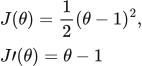
Differentiate the objective first
 LaTeX:
J(\theta)=\frac12(\theta-1)^2,\qquad J\prime(\theta)=\theta-1The power rule brings down 2, which cancels the half. The inside derivative is 1, so the remaining gradient is θ minus 1.
Update formulas
v stores the signed movement from the previous update. β = 0.9 retains 90% of that movement. Start v₀ = 0.
LaTeX: \theta_{\mathrm{look}}=\theta_{t-1}+\beta v_{t-1},\quad g_t=J\prime(\theta_{\mathrm{look}})LaTeX: v_t=\beta v_{t-1}-\eta g_t,\quad \theta_t=\theta_{t-1}+v_tStep 1: Update 1.
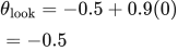 LaTeX:
\theta_{\mathrm{look}}=-0.5+0.9(0)=-0.5 LaTeX:
g_1=-0.5-(1)=-1.5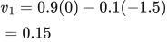 LaTeX:
v_1=0.9(0)-0.1(-1.5)=0.15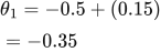 LaTeX:
\theta_1=-0.5+(0.15)=-0.35Step 2: Update 2.
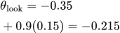 LaTeX:
\theta_{\mathrm{look}}=-0.35+0.9(0.15)=-0.215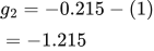 LaTeX:
g_2=-0.215-(1)=-1.215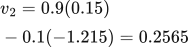 LaTeX:
v_2=0.9(0.15)-0.1(-1.215)=0.2565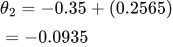 LaTeX:
\theta_2=-0.35+(0.2565)=-0.0935Final parameter after two updates: -0.0935. The lookahead locates the gradient; the new velocity is added to the old actual parameter, not to the lookahead.