Deep Learning · TEE · formulas

Batch normalization and learned scale/shift

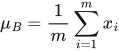
Batch normalization first uses batch statistics, then applies a learned scale and shift. Epsilon belongs inside the square root. Inference ordinarily uses stored running statistics.

$\mu_B=\frac{1}{m}\sum_{i=1}^{m}x_i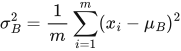$ LaTeX: \mu_B=\frac{1}{m}\sum_{i=1}^{m}x_i

$\sigma_B^2=\frac{1}{m}\sum_{i=1}^{m}(x_i-\mu_B)^2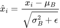$ LaTeX: \sigma_B^2=\frac{1}{m}\sum_{i=1}^{m}(x_i-\mu_B)^2

$\hat{x}_i=\frac{x_i-\mu_B}{\sqrt{\sigma_B^2+\epsilon}}$ LaTeX: \hat{x}_i=\frac{x_i-\mu_B}{\sqrt{\sigma_B^2+\epsilon}}

$y_i=\gamma\hat{x}_i+\beta$ LaTeX: y_i=\gamma\hat{x}_i+\beta

Batch normalization inside a residual network

Definition. Batch normalization normalizes a feature using training-batch statistics, then applies a learned scale and shift. It operates on intermediate activations and is different from normalizing the original dataset once before training.

For one feature with m values in a training batch:

$\mu_B=\frac{1}{m}\sum_{i=1}^{m}x_i$ LaTeX: \mu_B=\frac{1}{m}\sum_{i=1}^{m}x_i

$\sigma_B^2=\frac{1}{m}\sum_{i=1}^{m}(x_i-\mu_B)^2$ LaTeX: \sigma_B^2=\frac{1}{m}\sum_{i=1}^{m}(x_i-\mu_B)^2

$\hat{x}_i=\frac{x_i-\mu_B}{\sqrt{\sigma_B^2+\epsilon}}$ LaTeX: \hat{x}_i=\frac{x_i-\mu_B}{\sqrt{\sigma_B^2+\epsilon}}

$y_i=\gamma\hat{x}_i+\beta$ LaTeX: y_i=\gamma\hat{x}_i+\beta

The batch mean μ_B is the centre; batch variance σ²_B measures squared spread. Epsilon ε is a small positive stability constant inside the square root. Gamma γ is a learned scale and beta β is a learned shift. For convolutional BN, statistics are usually computed separately for each channel across batch and spatial positions. Ordinary inference uses stored running statistics rather than the current test batch.

Question (practice, 3 marks). For one feature, a training batch contains [2,4]. Use ε = 0.00001, γ = 2 and β = 0.5. Calculate both batch-normalized outputs using population variance.

Given

x₁ = 2; x₂ = 4; m = 2; ε = 0.00001; γ = 2; β = 0.5.

To find

Batch mean, variance, normalized values and scale-and-shift outputs.

Formula — which one and why

Use the four formulas above in order. Population variance divides by m = 2, not m − 1. Scale and shift follow normalization because the model can learn the useful final feature scale.

Solution — step by step

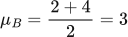
Step 1: mean.

$\mu_B=\frac{2+4}{2}=3$ LaTeX: \mu_B=\frac{2+4}{2}=3

Step 2: deviations. 2 − 3 = −1 and 4 − 3 = 1.

Step 3: squared deviations and variance.

$\sigma_B^2=\frac{(-1)^2+1^2}{2}=\frac{1+1}{2}=1$ LaTeX: \sigma_B^2=\frac{(-1)^2+1^2}{2}=\frac{1+1}{2}=1

Step 4: stable denominator.

$d=\sqrt{1+0.00001}\approx1.00000499999$ LaTeX: d=\sqrt{1+0.00001}\approx1.00000499999

Step 5: normalize separately.

$\hat{x}_1=\frac{-1}{d}\approx-0.99999500004$ LaTeX: \hat{x}_1=\frac{-1}{d}\approx-0.99999500004

$\hat{x}_2=\frac{1}{d}\approx0.99999500004$ LaTeX: \hat{x}_2=\frac{1}{d}\approx0.99999500004

Step 6: scale the first normalized value, then shift it.

$y_1=2(-0.99999500004)+0.5\approx-1.49999000008$ LaTeX: y_1=2(-0.99999500004)+0.5\approx-1.49999000008

Step 7: scale the second normalized value, then shift it.

$y_2=2(0.99999500004)+0.5\approx2.49999000008$ LaTeX: y_2=2(0.99999500004)+0.5\approx2.49999000008

Final answer: output ≈ [−1.49999,2.49999]. Its mean is β = 0.5; the final output need not have zero mean after the learned shift. The normalized values themselves have mean zero here.

Yaad rakho: centre hatao → spread se divide → learned scale lagao → shift add karo.