Deep Learning · TEE · formulas
Sigmoid and its derivative
Sigmoid takes a raw score and changes it to a number between 0 and 1. Its derivative is a different number: it tells backpropagation how sensitive that output is to its raw score. The complete example below calculates both and shows where each is used.
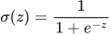 LaTeX:
\sigma(z)=\frac{1}{1+e^{-z}} LaTeX:
\sigma\prime(z)=\sigma(z)[1-\sigma(z)]Complete sigmoid training example
Question. A sigmoid neuron has input 2, weight 0, bias 0, target 1 and half squared loss. Will gradient descent increase or decrease the weight? Use learning rate 0.1 and calculate the exact update.
Given
x = 2; w = 0; b = 0; y = 1.
Sigmoid output; half squared loss; η = 0.1.
To find
Find the weight-gradient sign, exact weight update and resulting weight.
Formula — which one and why
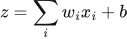
Weighted sum and activation. Each input is multiplied by its connection weight. Add these contributions, add the bias once, then apply the stated activation.
xᵢ = input i; wᵢ = its weight; b = bias; z = sum before activation; a = output after activation; f = the specified activation function.
 LaTeX:
z=\sum_iw_ix_i+b LaTeX:
a=f(z)Yaad rakhne ka cue: Input × weight, sabka sum, bias once, phir activation.
Sigmoid and its slope. Use sigmoid when the neuron is specified to squash its preactivation into (0,1). Once its output is known, its derivative needs only output × (1−output).
z = preactivation; p = sigmoid output; e is the exponential base, not a prediction error in this formula.
 LaTeX:
p=\frac{1}{1+e^{-z}}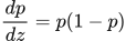 LaTeX:
\frac{dp}{dz}=p(1-p)Yaad rakhne ka cue: Sigmoid output p; uska slope p × (1−p).
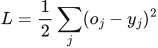
Half summed squared loss. This loss convention takes one-half of the sum of squared prediction errors. Use it when the question specifies it, or explicitly state it as an assumption when the paper omits the loss. Differentiating cancels the factor one-half against the square derivative.
oⱼ = output j; yⱼ = target j; L = half summed squared loss under the stated or explicitly assumed convention.
 LaTeX:
L=\frac12\sum_j(o_j-y_j)^2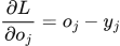 LaTeX:
\frac{\partial L}{\partial o_j}=o_j-y_jYaad rakhne ka cue: Half aur square ka 2 cancel: output derivative = prediction − target.
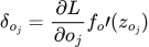
Backpropagation. The loss tells us how each output must change. Multiply by that neuron’s activation slope to obtain its delta. A weight gradient is receiving delta × sending value. Hidden deltas must include every outgoing path.
δ (delta) = derivative of loss with respect to a neuron’s preactivation; f′ = activation derivative; aᵢ = sending activation; Wⱼᵢ = connection weight. Use the exact loss scaling in the question.
 LaTeX:
\delta_{o_j}=\frac{\partial L}{\partial o_j}f_o\prime(z_{o_j})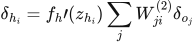 LaTeX:
\delta_{h_i}=f_h\prime(z_{h_i})\sum_jW_{ji}^{(2)}\delta_{o_j}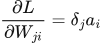 LaTeX:
\frac{\partial L}{\partial W_{ji}}=\delta_ja_i LaTeX:
\frac{\partial L}{\partial b_j}=\delta_j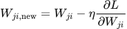 LaTeX:
W_{ji,\mathrm{new}}=W_{ji}-\eta\frac{\partial L}{\partial W_{ji}}Yaad rakhne ka cue: Receiving delta × sending value = us connection ka gradient.
Solution — step by step
Step 1 forward: net = 0(2) + 0 = 0; sigmoid output = 0.5.
Step 2 backward: prediction minus target = 0.5 − 1 = −0.5. Sigmoid slope = 0.5(1 − 0.5) = 0.25. Delta = −0.5 × 0.25 = −0.125.
Step 3 gradients and update: weight gradient = −0.125 × 2 = −0.25. New weight = 0 − 0.1(−0.25) = 0.025. Bias gradient = −0.125; new bias = 0.0125. Both increase. With positive input, these changes initially raise the prediction toward the target. Your intuition and arithmetic now agree.
Drill 10 Sigmoid neuron gradient
Question
Question. x = 2, w = 0.5, b = 0, y = 1, half squared loss, η = 0.1. Find one weight and bias update.
Answer — step by step
Given
x = 2; w = 0.5; b = 0; target y = 1.
Activation: sigmoid; loss: half squared error.
Learning rate η = 0.1.
To find
Find the output, delta, weight/bias gradients and one update.
Formula — which one and why
Weighted sum and activation. Each input is multiplied by its connection weight. Add these contributions, add the bias once, then apply the stated activation.
xᵢ = input i; wᵢ = its weight; b = bias; z = sum before activation; a = output after activation; f = the specified activation function.
LaTeX: z=\sum_iw_ix_i+bLaTeX: a=f(z)Yaad rakhne ka cue: Input × weight, sabka sum, bias once, phir activation.
Sigmoid and its slope. Use sigmoid when the neuron is specified to squash its preactivation into (0,1). Once its output is known, its derivative needs only output × (1−output).
z = preactivation; p = sigmoid output; e is the exponential base, not a prediction error in this formula.
LaTeX: p=\frac{1}{1+e^{-z}}LaTeX: \frac{dp}{dz}=p(1-p)Yaad rakhne ka cue: Sigmoid output p; uska slope p × (1−p).
Half summed squared loss. This loss convention takes one-half of the sum of squared prediction errors. Use it when the question specifies it, or explicitly state it as an assumption when the paper omits the loss. Differentiating cancels the factor one-half against the square derivative.
oⱼ = output j; yⱼ = target j; L = half summed squared loss under the stated or explicitly assumed convention.
LaTeX: L=\frac12\sum_j(o_j-y_j)^2LaTeX: \frac{\partial L}{\partial o_j}=o_j-y_jYaad rakhne ka cue: Half aur square ka 2 cancel: output derivative = prediction − target.
Backpropagation. The loss tells us how each output must change. Multiply by that neuron’s activation slope to obtain its delta. A weight gradient is receiving delta × sending value. Hidden deltas must include every outgoing path.
δ (delta) = derivative of loss with respect to a neuron’s preactivation; f′ = activation derivative; aᵢ = sending activation; Wⱼᵢ = connection weight. Use the exact loss scaling in the question.
LaTeX: \delta_{o_j}=\frac{\partial L}{\partial o_j}f_o\prime(z_{o_j})LaTeX: \delta_{h_i}=f_h\prime(z_{h_i})\sum_jW_{ji}^{(2)}\delta_{o_j}LaTeX: \frac{\partial L}{\partial W_{ji}}=\delta_ja_iLaTeX: \frac{\partial L}{\partial b_j}=\delta_jLaTeX: W_{ji,\mathrm{new}}=W_{ji}-\eta\frac{\partial L}{\partial W_{ji}}Yaad rakhne ka cue: Receiving delta × sending value = us connection ka gradient.
Solution — step by step
Meaning and formulas
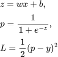
Here the loss is half squared error. It is different from binary cross-entropy, so we include the sigmoid derivative explicitly.
 LaTeX:
z=wx+b,\quad p=\frac1{1+e^{-z}},\quad L=\frac12(p-y)^2The symbol δ (delta) is a short name for the loss gradient with respect to the neuron's raw score z.
 LaTeX:
\delta=(p-y)p(1-p)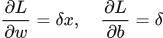 LaTeX:
\frac{\partial L}{\partial w}=\delta x,\quad \frac{\partial L}{\partial b}=\delta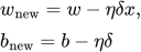 LaTeX:
w_{\mathrm{new}}=w-\eta\delta x,\quad b_{\mathrm{new}}=b-\eta\deltaStep 1: weighted sum and sigmoid
 LaTeX:
z=0.5\times2+0=1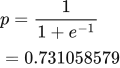 LaTeX:
p=\frac1{1+e^{-1}}=0.731058579Step 2: error and activation slope
 LaTeX:
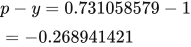
p-y=0.731058579-1=-0.268941421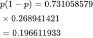 LaTeX:
p(1-p)=0.731058579\times0.268941421=0.196611933Step 3: multiply the linked effects to obtain delta
 LaTeX:
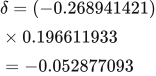
\delta=(-0.268941421)\times0.196611933=-0.052877093Step 4: multiply delta by the input to each parameter
The weight receives x = 2. The bias effectively receives the constant input 1.
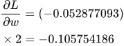 LaTeX:
\frac{\partial L}{\partial w}=(-0.052877093)\times2=-0.105754186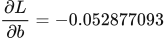 LaTeX:
\frac{\partial L}{\partial b}=-0.052877093Step 5: subtract learning rate times each gradient
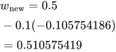 LaTeX:
w_{\mathrm{new}}=0.5-0.1(-0.105754186)=0.510575419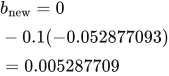 LaTeX:
b_{\mathrm{new}}=0-0.1(-0.052877093)=0.005287709Final answer: new weight ≈ 0.510575419; new bias ≈ 0.005287709. Subtracting negative gradients increases both values here.
sigmoid example 1
Question. For preactivation z = -2, calculate the sigmoid output and state its derivative.
Given
z = -2; activation = sigmoid.
To find
The output a and the derivative with respect to z.
Formula — which one and why
Use the activation named in the question. The derivative is a second calculation required for a backward pass.
z is the raw sum; a is the activated output; f′(z) is the local slope.
 LaTeX:
a=\frac1{1+e^{-z}} LaTeX:
f\prime(z)=a(1-a)Yaad rakhne ka cue: One over one plus e ki minus-z power; slope = output × (1−output).
Solution — step by step
Step 1: negate the whole input.
 LaTeX:
-z=-(-2)=2Step 2: calculate the exponential.
 LaTeX:
e^{2}\approx7.389056099Step 3: add one in the denominator.
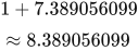 LaTeX:
1+7.389056099\approx8.389056099Step 4: divide one by the complete denominator.
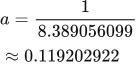 LaTeX:
a=\frac1{8.389056099}\approx0.119202922Step 5: use the activated output in the slope.
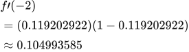 LaTeX:
f\prime(-2)=(0.119202922)(1-0.119202922)\approx0.104993585Final answer: a ≈ 0.119202922. Derivative ≈ 0.104993585.
sigmoid example 2
Question. For preactivation z = 0, calculate the sigmoid output and state its derivative.
Given
z = 0; activation = sigmoid.
To find
The output a and the derivative with respect to z.
Formula — which one and why
Use the activation named in the question. The derivative is a second calculation required for a backward pass.
z is the raw sum; a is the activated output; f′(z) is the local slope.
LaTeX: a=\frac1{1+e^{-z}}LaTeX: f\prime(z)=a(1-a)Yaad rakhne ka cue: One over one plus e ki minus-z power; slope = output × (1−output).
Solution — step by step
Step 1: negate the whole input.
 LaTeX:
-z=-(0)=0Step 2: calculate the exponential.
 LaTeX:
e^{0}\approx1.000000000Step 3: add one in the denominator.
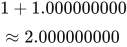 LaTeX:
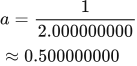
1+1.000000000\approx2.000000000Step 4: divide one by the complete denominator.
 LaTeX:
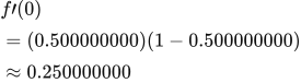
a=\frac1{2.000000000}\approx0.500000000Step 5: use the activated output in the slope.
 LaTeX:
f\prime(0)=(0.500000000)(1-0.500000000)\approx0.250000000Final answer: a ≈ 0.500000000. Derivative ≈ 0.250000000.
sigmoid example 3
Question. For preactivation z = 2, calculate the sigmoid output and state its derivative.
Given
z = 2; activation = sigmoid.
To find
The output a and the derivative with respect to z.
Formula — which one and why
Use the activation named in the question. The derivative is a second calculation required for a backward pass.
z is the raw sum; a is the activated output; f′(z) is the local slope.
LaTeX: a=\frac1{1+e^{-z}}LaTeX: f\prime(z)=a(1-a)Yaad rakhne ka cue: One over one plus e ki minus-z power; slope = output × (1−output).
Solution — step by step
Step 1: negate the whole input.
 LaTeX:
-z=-(2)=-2Step 2: calculate the exponential.
 LaTeX:
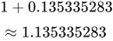
e^{-2}\approx0.135335283Step 3: add one in the denominator.
 LaTeX:
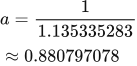
1+0.135335283\approx1.135335283Step 4: divide one by the complete denominator.
 LaTeX:
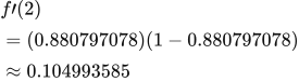
a=\frac1{1.135335283}\approx0.880797078Step 5: use the activated output in the slope.
 LaTeX:
f\prime(2)=(0.880797078)(1-0.880797078)\approx0.104993585Final answer: a ≈ 0.880797078. Derivative ≈ 0.104993585.