Deep Learning · TEE · mocks
MT2 Mock A
60 minutes · 10 marks. Q1(a,b): 2 marks each, compulsory; attempt any two of Q2–Q4: 3 marks each. This uses the shared M2 choice pattern already supplied. The latest faculty message guides the Unit 3–4 theory/numerical mix; it does not fix individual question numbers or numerical topics. Q1 theory · two Unit 4 numericals + Unit 3 theory among the 3-mark choices
Q1a
Question
Q1a compulsory (2 marks). Explain the key difference between the AdaGrad and RMSProp accumulators. Why can AdaGrad's effective learning rate become very small during prolonged training?
Answer — step by step
1. AdaGrad stores a running sum
Let gₜ be the current gradient and Gₜ the stored sum of squared gradients. AdaGrad updates that sum as follows:
 LaTeX:
G_t=G_{t-1}+g_t^2Every added square is nonnegative, so G cannot decrease. All past squared gradients remain in the sum.
2. RMSProp stores a decaying average
Let sₜ be the stored squared-gradient average and ρ the fraction of the previous average retained.
 LaTeX:
s_t=\rho s_{t-1}+(1-\rho)g_t^2RMSProp gradually reduces the influence of older squared gradients. Its accumulator can rise or fall, depending on the new squared gradient.
3. Explain the effect on step size
AdaGrad's effective learning rate is:
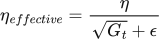 LaTeX:
\eta_{effective}=\frac{\eta}{\sqrt{G_t}+\epsilon}Here η is the base learning rate and ε is a small positive number that stabilizes division. When G becomes large, its square root becomes large, so dividing by it produces a smaller effective learning rate. RMSProp's decaying average avoids this particular permanent-accumulation problem.
Final answer: AdaGrad uses a nondecreasing sum of all squared gradients; RMSProp uses a decaying average. AdaGrad's growing denominator can make future updates very small.
Yaad rakho: AdaGrad sab squares jodta rehta hai; RMSProp purane squares ka asar dheere kam karta hai.
Q1b
Question
Q1b compulsory (2 marks). Explain local connectivity and parameter sharing in a CNN. How do they reduce the number of learned parameters compared with a fully connected mapping of an image?
Answer — step by step
1. Local connectivity
Each convolutional output depends on a small spatial neighbourhood of the input, called its receptive field, rather than every pixel in the entire image. The filter spans the input channels within that neighbourhood. This limits the connections used to calculate each output.
2. Parameter sharing
The same filter weights and bias are reused at every spatial position where that filter is applied. A CNN therefore learns one set of parameters for that filter, rather than a separate set for each image location.
3. Concrete image example
An edge-detecting filter can identify a vertical boundary near the left of an image and then slide to look for a similar boundary near the right. Both locations use the same learned filter. The network does not need to learn an independent edge detector for every position.
4. Comparison with a fully connected mapping
A fully connected layer generally learns a separate weight for every input-to-output connection. Convolution reduces this requirement in two ways: local connectivity restricts each output's input region, while parameter sharing reuses one filter across locations. More output positions create more activations and computation, but do not create new parameters for that shared filter.
Final answer: local connectivity uses a limited input neighbourhood; parameter sharing reuses the filter's learned values across spatial positions. Together they can require far fewer parameters than a fully connected image mapping.
Yaad rakho: Filter ke numbers ek baar seekhte hain; image par baar-baar wahi use hote hain.
Q2
Question
Q2 optional (3 marks). An input of size 7 × 7 × 3 passes through a convolutional layer with two 3 × 3 filters, stride 2 and padding 1 on each side; then a 2 × 2 pooling layer with stride 2 and no padding; then flattening; then a dense layer with three output units. Find the output shape after every layer and the total trainable parameters. Include one bias per convolutional filter and per dense unit.
Answer — step by step
Given
- Input: height 7, width 7, channels 3.
- Convolution: kernel 3 × 3, filters 2, stride 2, padding 1 per side.
- Pooling: window 2 × 2, stride 2, padding 0.
- Flattening followed by 3 dense output units.
- Include all specified biases. Pooling and flattening have no learned parameters.
To find
The convolution output, pooling output, flatten length, dense output length and total trainable parameter count.
Formula — which one and why
For either spatial axis, use the output-size formula. N is that axis's input size, K the window size, S its stride and P padding per side. The floor means discard any fractional part because a full window must fit.
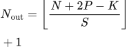 LaTeX:
N_{\mathrm{out}}=\left\lfloor\frac{N+2P-K}{S}\right\rfloor+1Each convolution filter spans all input channels; each dense unit connects to every flattened input. Therefore:
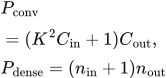 LaTeX:
P_{\mathrm{conv}}=(K^2C_{\mathrm{in}}+1)C_{\mathrm{out}},\qquad P_{\mathrm{dense}}=(n_{\mathrm{in}}+1)n_{\mathrm{out}}Flattening simply counts all values in the preceding feature maps:
 LaTeX:
n_{\mathrm{flat}}=HWCSolution — step by step
Step 1: convolution height and width
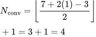 LaTeX:
N_{\mathrm{conv}}=\left\lfloor\frac{7+2(1)-3}{2}\right\rfloor+1=3+1=4The numerator is 7 + 2 − 3 = 6. Divide by stride 2 to get 3, then add 1 to get 4 positions. The same calculation applies to height and width. Two filters create two output channels.
Convolution output: 4 × 4 × 2.
Step 2: convolution parameters
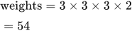 LaTeX:
\text{weights}=3\times3\times3\times2=54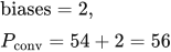 LaTeX:
\text{biases}=2,\qquad P_{\mathrm{conv}}=54+2=56Step 3: pooling shape and parameters
The pooling input size is now 4, not the original 7.
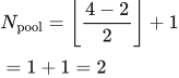 LaTeX:
N_{\mathrm{pool}}=\left\lfloor\frac{4-2}{2}\right\rfloor+1=1+1=2Pooling operates separately on each channel, so the two channels remain two.
Pooling output: 2 × 2 × 2. Pooling parameters: 0.
Step 4: flattening
 LaTeX:
n_{\mathrm{flat}}=2\times2\times2=8There are eight values to send to the dense layer. Flattening rearranges them into a list and learns no parameters.
Flatten output: 8 values. Flatten parameters: 0.
Step 5: dense output and parameters
Each of the three dense units receives eight inputs and has one bias.
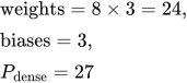 LaTeX:
\text{weights}=8\times3=24,\quad\text{biases}=3,\quad P_{\mathrm{dense}}=27Dense output: 3 values.
Step 6: total trainable parameters
 LaTeX:
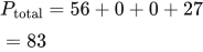
P_{\mathrm{total}}=56+0+0+27=83Final answer: 4 × 4 × 2 → 2 × 2 × 2 → 8 → 3. Total: 83 trainable parameters.
Yaad rakho: Pehle shape; phir weights. Ek layer ka output hi next layer ka input hai.
Q3
Question
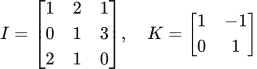
Q3 optional (3 marks). Apply the printed kernel K to input I using the deep-learning cross-correlation convention, with stride 1, no padding and zero bias. Do not flip K. Apply ReLU to the resulting map, followed by 2 × 2 max pooling with stride 2 and no padding. Show every convolution entry and find the final output.
 LaTeX:
I=\begin{bmatrix}1&2&1\\0&1&3\\2&1&0\end{bmatrix},\quad K=\begin{bmatrix}1&-1\\0&1\end{bmatrix}Answer — step by step
Given
- Input I is the printed 3 × 3 matrix; kernel K is the printed 2 × 2 matrix.
- Convolution stride 1, padding 0, bias 0; use K in its printed orientation.
- Activation: ReLU.
- Pooling: max, 2 × 2 window, stride 2, padding 0.
To find
All four convolution values, the ReLU output matrix and the final pooled output.
Formula — which one and why
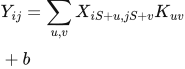
For each input window, multiply entries at matching positions, then add all products and the bias once.
 LaTeX:
Y_{ij}=\sum_{u,v}X_{iS+u,jS+v}K_{uv}+bX is the input, S is stride, u and v select a kernel entry, and b is bias. This formula uses zero-based array indices; the written solution labels positions from 1 for readability.
ReLU is required because the question requests activation after convolution. It replaces a negative value by zero.
 LaTeX:
\operatorname{ReLU}(z)=\max(0,z)Max pooling selects the largest value in its current window V.
 LaTeX:
y_{\max}=\max VSolution — step by step
Follow each selected input window below. Matching row colors connect its input cells, kernel coefficients and products; the outlined output cell shows where their sum belongs.
Step 1: determine the convolution shape
For each axis: (3 − 2)/1 + 1 = 2. Therefore calculate a 2 × 2 output matrix.
Step 2: top-left output, position (1,1)
The window is  LaTeX:
\begin{bmatrix}1 & 2\\0 & 1\end{bmatrix}.
Multiply matching cells: 1 × 1 = 1; 2 × (−1) = −2; 0 × 0 = 0; 1 × 1 = 1.
Add the products and bias: 1 − 2 + 0 + 1 + 0 = 0.
Step 3: top-right output, position (1,2)
Move the window one column to the right. The window is  LaTeX:
\begin{bmatrix}2 & 1\\1 & 3\end{bmatrix}.
Multiply matching cells: 2 × 1 = 2; 1 × (−1) = −1; 1 × 0 = 0; 3 × 1 = 3.
Add: 2 − 1 + 0 + 3 + 0 = 4.
Step 4: bottom-left output, position (2,1)
The window is  LaTeX:
\begin{bmatrix}0 & 1\\2 & 1\end{bmatrix}.
Multiply matching cells: 0 × 1 = 0; 1 × (−1) = −1; 2 × 0 = 0; 1 × 1 = 1.
Add: 0 − 1 + 0 + 1 + 0 = 0.
Step 5: bottom-right output, position (2,2)
The window is  LaTeX:
\begin{bmatrix}1 & 3\\1 & 0\end{bmatrix}.
Multiply matching cells: 1 × 1 = 1; 3 × (−1) = −3; 1 × 0 = 0; 0 × 1 = 0.
Add: 1 − 3 + 0 + 0 + 0 = −2.
Convolution map:  LaTeX:
\begin{bmatrix}0 & 4\\0 & -2\end{bmatrix}.
Step 6: apply ReLU separately to every entry
- max(0,0) = 0.
- max(0,4) = 4.
- max(0,0) = 0.
- max(0,−2) = 0.
ReLU map:  LaTeX:
\begin{bmatrix}0 & 4\\0 & 0\end{bmatrix}.
Step 7: max pooling
The 2 × 2 pooling window covers all four activated entries. Compare 0, 4, 0 and 0. Their maximum is 4.
Final answer: convolution LaTeX: \begin{bmatrix}0 & 4\\0 & -2\end{bmatrix} → ReLU LaTeX: \begin{bmatrix}0 & 4\\0 & 0\end{bmatrix} → pooled output  LaTeX:
\begin{bmatrix}4\end{bmatrix}, a 1 × 1 map.
Yaad rakho: Multiply-add se convolution; negative hatao ReLU; biggest uthao max pool.
Q4
Question
Q4 optional (3 marks). What is overfitting? Explain how dropout and early stopping help improve generalization. State which dataset should select the stopping point.
Answer — step by step
1. Definition and identification
Overfitting occurs when a model learns training-specific details or noise that do not generalize to new data. It commonly shows low training error together with substantially higher validation error. Generalization means performing well on new examples drawn from the task's data distribution.
2. Dropout
During training, dropout randomly sets selected activations to zero. The active subnetwork changes across training passes, discouraging reliance on a fixed combination of hidden units. Under inverted dropout, retained activations are divided by the keep probability to preserve their expected scale. During ordinary inference, the masking is disabled and all units are used without that training-time rescaling.
Dropout is a regularizer; it can reduce overfitting, but excessive dropout can cause underfitting.
3. Early stopping
Train on the training set and monitor performance on a separate validation set. Save the model whenever validation loss improves. Stop after the chosen number of consecutive non-improving evaluations, called patience, then restore the saved best model.
For example, validation losses 0.8, 0.6, 0.5, 0.53 and 0.55 have their minimum at epoch 3. With patience 2, stop after epoch 5 and restore epoch 3. The stopping epoch and saved-model epoch are different.
Final answer: dropout restricts dependence on particular training-time activations; early stopping limits training after validation performance stops improving. Choose the stopping point using validation data and reserve the test set for final evaluation.
Yaad rakho: Training se seekho, validation se best model chuno, test se final result batao.