Deep Learning · TEE · mocks
MT2 Mock B
60 minutes · 10 marks. Q1(a,b): 2 marks each, compulsory; attempt any two of Q2–Q4: 3 marks each. This uses the shared M2 choice pattern already supplied. The latest faculty message guides the Unit 3–4 theory/numerical mix; it does not fix individual question numbers or numerical topics. Q1 theory/numerical combination · Unit 3 theory + numerical mixed question, Unit 4 numerical, Unit 4 theory
Q1a
Question
Q1a compulsory (2 marks). Explain the purpose of scaling retained activations in inverted dropout. For activations [1,2,3,4], keep probability 0.5 and mask [1,0,1,0], calculate the activations used during this training pass. A mask value of 1 means keep and 0 means drop.
Answer — step by step
Theory: why scale retained values?
Randomly dropping units would reduce the average activation. Inverted dropout divides every retained activation by the keep probability. Averaged over the random masks, this preserves the original activation's expected value. A dropped activation is still zero.
Given
- Original activations a = [1,2,3,4].
- Keep probability q = 0.5, meaning a unit has a 50% chance of being kept.
- This pass's supplied mask m = [1,0,1,0].
To find
The four post-dropout activations used in this training pass.
Formula — which one and why
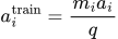
Multiply the original activation aᵢ by its mask mᵢ, then divide by keep probability q.
 LaTeX:
a_i^{\mathrm{train}}=\frac{m_ia_i}{q}Solution — step by step
Step 1: first activation
Mask 1 keeps the value. Multiply 1 × 1 = 1; divide 1 by 0.5 to get 2.
Step 2: second activation
Mask 0 drops the value. Multiply 0 × 2 = 0; divide 0 by 0.5 to get 0.
Step 3: third activation
Mask 1 keeps the value. Multiply 1 × 3 = 3; divide 3 by 0.5 to get 6.
Step 4: fourth activation
Mask 0 drops the value. Multiply 0 × 4 = 0; divide 0 by 0.5 to get 0.
Final answer: [2,0,6,0]. This is the training-pass result. In ordinary inference with inverted dropout, disable the mask and its scaling.
Yaad rakho: Mask lagao; bache hue values ko keep probability se divide karo.
Q1b
Question
Q1b compulsory (2 marks). Explain a ResNet shortcut. Why must the two tensors being added have matching shapes, and what can be done if their shapes differ?
Answer — step by step
1. Residual addition
A residual block combines a learned transformation F(x) with a shortcut carrying the input x:
 LaTeX:
H(x)=F(x)+xF(x) is the output of the learned residual branch. Adding x provides a direct path for information and gradients, helping optimize deep networks. If the branch produces zero, the addition stage returns x. A post-addition activation, if specified by the architecture, is applied afterward.
2. Why matching shapes are needed
The addition is entry by entry. Each element in F(x) needs a corresponding element in x, so height, width and channel count must match. For example, a 14 × 14 × 32 tensor cannot be directly added to a 14 × 14 × 64 tensor in a standard residual shortcut.
3. How a projection helps
A learned projection, commonly a 1 × 1 convolution with an appropriate number of filters and stride, maps the shortcut to the required shape. Then add the projected shortcut and the residual branch. This is addition, not channel concatenation.
Final answer: a shortcut adds input information to the learned residual branch. Use an identity shortcut when shapes match and a suitable projection when they do not.
Yaad rakho: Same-size entries jodte hain; mismatch ho toh shortcut ka size pehle match karo.
Q2
Question
Q2 optional (3 marks). (a) Explain why Adam uses bias correction for its initially zero moment estimates. (1 mark) (b) Adam starts with θ₀ = 1 and m₀ = v₀ = 0. Use learning rate η = 0.1, β₁ = 0.9 and β₂ = 0.99. The supplied gradients are g₁ = 2 and g₂ = −1. Perform two bias-corrected updates. Show the raw first and second moments, corrected moments and updated parameter after each iteration. Set ε = 0 only for this nonzero-denominator hand calculation. (2 marks)
Answer — step by step
Part (a): why Adam corrects the moments
Adam initializes both moving averages to zero. At early iterations, too little gradient history has accumulated, so the raw estimates are biased toward zero. Dividing mₜ by 1 − β₁ᵗ and vₜ by 1 − β₂ᵗ corrects this initialization bias before the parameter update. The power uses the current iteration number t. As t increases, these denominators approach 1.
Part (b): numerical solution
Given
- Starting parameter θ₀ = 1.
- Starting first moment m₀ = 0 and second moment v₀ = 0.
- Learning rate η = 0.1.
- Decay factors β₁ = 0.9 and β₂ = 0.99.
- Supplied gradients, in order: 2, then −1.
- ε = 0 for this exercise; both denominators will be nonzero.
To find
For iterations 1 and 2, calculate m, v, their bias-corrected values and the new parameter θ.
Formula — which one and why
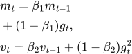
Adam keeps two moving averages: m stores signed gradients and v stores squared gradients. Zero initialization makes these averages initially too small, so divide by the correction factors for the current iteration t.
 LaTeX:
m_t=\beta_1m_{t-1}+(1-\beta_1)g_t,\quad v_t=\beta_2v_{t-1}+(1-\beta_2)g_t^2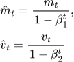 LaTeX:
\hat m_t=\frac{m_t}{1-\beta_1^t},\quad\hat v_t=\frac{v_t}{1-\beta_2^t}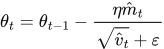 LaTeX:
\theta_t=\theta_{t-1}-\frac{\eta\hat m_t}{\sqrt{\hat v_t}+\varepsilon}The hat marks a corrected value. Carry the raw m and v into the next moving-average recurrence, not the corrected values. Keep full calculator precision until the final answer.
Solution — step by step
Step 1: iteration 1, raw first moment
The current gradient is 2. Retain 90% of the old first moment and add 10% of this gradient.
 LaTeX:
m_1=0.9(0)+0.1(2)=0.2Step 2: iteration 1, raw second moment
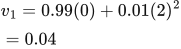
Square the gradient first: 2² = 4. Retain 99% of the old second moment and add 1% of that square.
 LaTeX:
v_1=0.99(0)+0.01(2)^2=0.04Step 3: iteration 1, bias correction
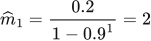
Use t = 1. The correction denominators are 1 − 0.9 = 0.1 and 1 − 0.99 = 0.01.
 LaTeX:
\widehat m_1=\frac{0.2}{1-0.9^{1}}=2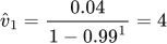 LaTeX:
\widehat v_1=\frac{0.04}{1-0.99^{1}}=4Step 4: iteration 1, parameter update
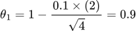
The square root of the corrected second moment is √4 = 2. The step is 0.1 × 2 ÷ 2 = 0.1.
 LaTeX:
\theta_1=1-\frac{0.1\times(2)}{\sqrt{4}}=0.9Step 5: iteration 2, raw first moment
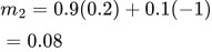
Use supplied gradient −1, previous raw m = 0.2 and previous raw v = 0.04.
 LaTeX:
m_2=0.9(0.2)+0.1(-1)=0.08The two contributions are 0.18 and −0.1; their sum is 0.08.
Step 6: iteration 2, raw second moment
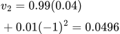
The square of −1 is +1.
 LaTeX:
v_2=0.99(0.04)+0.01(-1)^2=0.0496The two contributions are 0.0396 and 0.01; their sum is 0.0496.
Step 7: iteration 2, bias correction
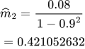
Use t = 2. The correction denominators are 1 − 0.9² = 0.19 and 1 − 0.99² = 0.0199.
 LaTeX:
\widehat m_2=\frac{0.08}{1-0.9^{2}}=0.421052632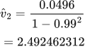 LaTeX:
\widehat v_2=\frac{0.0496}{1-0.99^{2}}=2.492462312Step 8: iteration 2, parameter update
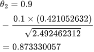
Start from the updated parameter 0.9. Take the square root of the corrected second moment, divide the corrected first moment by it, multiply by 0.1 and subtract.
 LaTeX:
\theta_2=0.9-\frac{0.1\times(0.421052632)}{\sqrt{2.492462312}}=0.873330057The displayed decimals are rounded; evaluate using the unrounded fractions when possible.
Final answer: θ₁ = 0.9 and θ₂ ≈ 0.873330057. The second supplied gradient is negative, but the first-moment estimate is still positive because it retains part of the previous positive gradient.
Yaad rakho: Do raw memories banao → current t se hats nikalo → update; next round mein raw memories le jao.
Q3
Question
Q3 optional (3 marks). A 16 × 16 × 64 feature map is processed by 32 filters of size 3 × 3 using stride 1 and same padding. Compare the direct convolution's MAC count with a bottleneck that first applies eight 1 × 1 filters, then the same 32-filter 3 × 3 convolution. Both stages keep spatial size 16 × 16. Find both costs, the absolute saving and percentage saving. Count one multiply–accumulate as one MAC and omit bias additions.
Answer — step by step
Given
- Input map: 16 × 16 with 64 channels.
- Direct layer: 32 filters, each 3 × 3, receiving 64 channels.
- Bottleneck stage 1: eight 1 × 1 filters, receiving 64 channels.
- Bottleneck stage 2: 32 filters, each 3 × 3, now receiving only 8 channels.
- Every layer has output height and width 16; ignore bias additions.
To find
Direct MACs, both bottleneck-stage MACs, their total, absolute saving and saving percentage.
Formula — which one and why
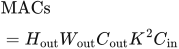
Each output entry uses K²Cᵢₙ weight–input pairs. There are HₒᵤₜWₒᵤₜCₒᵤₜ output entries. Multiply these counts:
 LaTeX:
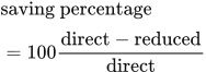
\mathrm{MACs}=H_{\mathrm{out}}W_{\mathrm{out}}C_{\mathrm{out}}K^2C_{\mathrm{in}}The bottleneck has two layers, so calculate each layer's work and add them. Saving is direct work minus reduced work, expressed as a fraction of direct work.
 LaTeX:
\mathrm{saving\ percentage}=100\frac{\mathrm{direct}-\mathrm{reduced}}{\mathrm{direct}}Solution — step by step
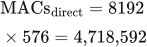
Step 1: direct convolution
Each output entry uses 3 × 3 × 64 = 576 weight–input pairs.
There are 16 × 16 × 32 = 8,192 output entries.
 LaTeX:
\mathrm{MACs}_{\mathrm{direct}}=8192\times576=4{,}718{,}592Step 2: 1 × 1 bottleneck reduction
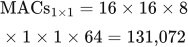
Each reduction output uses 1 × 1 × 64 = 64 weight–input pairs.
There are 16 × 16 × 8 = 2,048 reduction outputs.
 LaTeX:
\mathrm{MACs}_{1\times1}=16\times16\times8\times1\times1\times64=131{,}072The new map is 16 × 16 × 8. This changes the next layer's input channels to 8.
Step 3: following 3 × 3 convolution
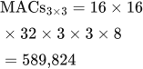
Each output now uses 3 × 3 × 8 = 72 weight–input pairs, instead of 576.
The number of outputs remains 16 × 16 × 32 = 8,192.
 LaTeX:
\mathrm{MACs}_{3\times3}=16\times16\times32\times3\times3\times8=589{,}824Step 4: total bottleneck cost
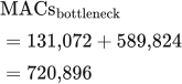
Include both stages; do not compare the direct layer against only the second stage.
 LaTeX:
\mathrm{MACs}_{\mathrm{bottleneck}}=131{,}072+589{,}824=720{,}896Step 5: absolute saving
 LaTeX:
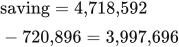
\mathrm{saving}=4{,}718{,}592-720{,}896=3{,}997{,}696Step 6: percentage saving
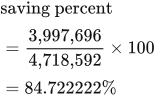
Divide the saving by the original direct cost, then multiply by 100.
 LaTeX:
\mathrm{saving\ percent}=\frac{3{,}997{,}696}{4{,}718{,}592}\times100=84.722222\%Final answer: direct 4,718,592 MACs; bottleneck 720,896 MACs; saving 3,997,696 MACs, approximately 84.72%. Both routes end in a 16 × 16 × 32 output, though they are different learned transformations.
Yaad rakho: 1 × 1 se channels kam; expensive 3 × 3 ka kaam kam. Dono stages ka cost jodna hai.
Q4
Question
Q4 optional (3 marks). Explain transfer learning for image classification with limited labelled data. Distinguish feature extraction from fine-tuning and describe a suitable training procedure.
Answer — step by step
1. Definition
Transfer learning reuses knowledge learned on a source task to help solve a target task. For image classification, a pretrained CNN can provide visual features that a new classifier uses for the target classes. This can reduce the amount of target data and training needed, provided the source features are useful for the target task.
2. Feature extraction and fine-tuning
| Method | Which parameters learn? | Main effect |
|---|---|---|
| Feature extraction | Keep pretrained backbone weights fixed; train a new classification head | Learn to classify using fixed pretrained features |
| Fine-tuning | Update selected pretrained layers as well as the new head | Adapt representations to the target task |
Freezing a layer stops its parameter updates; it does not remove its stored weights. Fine-tuning typically exposes more trainable parameters and therefore needs particular care with small datasets.
3. Training procedure
1. Create separate training, validation and test splits for the target problem.
2. Choose a suitable pretrained CNN and apply its required input size and preprocessing.
3. Replace the original classifier with a new head matching the target classes.
4. Freeze the backbone and train the new head on the training set.
5. If validation results justify it, unfreeze selected later layers and continue with an appropriately smaller learning rate.
6. Select the best checkpoint using validation performance; evaluate the final model on the held-out test set.
4. Concrete example
For a small dataset containing cats and dogs, reuse a pretrained image backbone and replace its original classifier with a binary-classification head. First learn the new head with the backbone frozen. Later, selected high-level layers may be fine-tuned if this improves validation performance.
Final answer: feature extraction learns a new classifier over fixed features; fine-tuning also adapts selected pretrained features. The correct choice depends on target data quantity, similarity to the source data and validation results.
Yaad rakho: Freeze mein purane features fixed; fine-tune mein selected purane features bhi seekhte hain.