Deep Learning · TEE · section
MT1B Q4
Current MT1 and the two teacher backprop examples
Question
Question (3 marks). Input x = [3]. Each row below lists the incoming weights of one receiving neuron. W₁ is shown below; b₁ = [0.2]; W₂ is shown below; b₂ = [0.1]. Hidden and output activations are sigmoid. Target y = [1]. Use L = ½(o−y)². Calculate the gradients of the output weight and output bias.
Answer — step by step
Given
Input x = [3].
W₁ is printed with the question.
b₁ = [0.2].
W₂ is printed with the question.
b₂ = [0.1].
Hidden and output activations are sigmoid.
Target y = [1].
To find
Find all preactivations, hidden activations and final outputs. Find the sigmoid output and, if requested, its derivative. Find the requested deltas and parameter gradients, then update the specified parameters.
Formula — which one and why
Forward propagation. Evaluate one layer completely before supplying its activated outputs to the next layer. Each layer has its own weights and biases.
x = input vector; h = hidden outputs; W₁,b₁ = hidden parameters; W₂,b₂ = output parameters; f₁,f₂ = the stated activations.
 LaTeX:
z_h=W_1x+b_1 LaTeX:
h=f_1(z_h) LaTeX:
z_o=W_2h+b_2 LaTeX:
o=f_2(z_o)Yaad rakhne ka cue: Pehli layer ka activated output hi agli layer ka input hai.
Sigmoid and its slope. Use sigmoid when the neuron is specified to squash its preactivation into (0,1). Once its output is known, its derivative needs only output × (1−output).
z = preactivation; p = sigmoid output; e is the exponential base, not a prediction error in this formula.
 LaTeX:
p=\frac{1}{1+e^{-z}}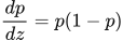 LaTeX:
\frac{dp}{dz}=p(1-p)Yaad rakhne ka cue: Sigmoid output p; uska slope p × (1−p).
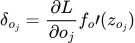
Backpropagation. The loss tells us how each output must change. Multiply by that neuron’s activation slope to obtain its delta. A weight gradient is receiving delta × sending value. Hidden deltas must include every outgoing path.
δ (delta) = derivative of loss with respect to a neuron’s preactivation; f′ = activation derivative; aᵢ = sending activation; Wⱼᵢ = connection weight. Use the exact loss scaling in the question.
 LaTeX:
\delta_{o_j}=\frac{\partial L}{\partial o_j}f_o\prime(z_{o_j})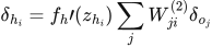 LaTeX:
\delta_{h_i}=f_h\prime(z_{h_i})\sum_jW_{ji}^{(2)}\delta_{o_j}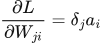 LaTeX:
\frac{\partial L}{\partial W_{ji}}=\delta_ja_i LaTeX:
\frac{\partial L}{\partial b_j}=\delta_j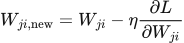 LaTeX:
W_{ji,\mathrm{new}}=W_{ji}-\eta\frac{\partial L}{\partial W_{ji}}Yaad rakhne ka cue: Receiving delta × sending value = us connection ka gradient.
Solution — step by step
Step 1 map the arrows. Each row of W₁ receives all inputs; each row of W₂ receives all hidden outputs. Bias is added once per receiving neuron. All gradients below use the OLD weights from this same forward pass.
Hidden neuron 1:
 LaTeX:
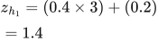
z_{h_1} = (0.4 \times 3) + (0.2) = 1.4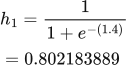 LaTeX:
h_{1}=\frac{1}{1+e^{-(1.4)}}=0.802183889Output neuron 1:
 LaTeX:
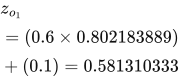
z_{o_1} = (0.6 \times 0.802183889) + (0.1) = 0.581310333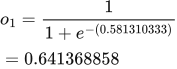 LaTeX:
o_{1}=\frac{1}{1+e^{-(0.581310333)}}=0.641368858Step 2 loss convention. Use the half squared loss stated in this question. No learning rate is supplied.
Prediction minus target = [-0.358631142]. Squared errors = [0.128616296]. Half-sum squared loss = 0.064308148; mean squared error = 0.128616296. These are different unless the number of output components makes the scale coincide.
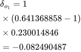
Output delta 1:
 LaTeX:
\delta_{o_1} = 1 \times (0.641368858-1) \times 0.230014846 = -0.082490487The derivative is o(1−o).
Step 3 output weights. Gradient = receiving delta × sending activation. An output bias gradient equals its delta.
h1 → o1:
The sending value and receiving delta have different roles. All deltas still use the original forward-pass weights.
The receiving neuron supplies the delta; the sending neuron supplies its activation.
 LaTeX:
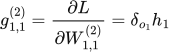
g_{1,1}^{(2)}=\frac{\partial L}{\partial W^{(2)}_{1,1}}=\delta_{o_1}h_1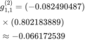 LaTeX:
g_{1,1}^{(2)}=(-0.082490487)\times(0.802183889)\approx -0.066172539Step 4 hidden deltas. A hidden unit can influence EVERY connected output, so add those paths BEFORE multiplying by the hidden activation derivative.
Hidden 1 downstream contribution:
Calculate each outgoing path using the old outgoing weight and that output's delta.
Multiply within each path. Add the resulting contributions at the shared hidden neuron.
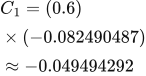
Contribution from output 1.
 LaTeX:
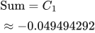
C_1=(0.6)\times(-0.082490487)\approx -0.049494292Accumulate the contributions, then apply the hidden activation derivative below.
 LaTeX:
\text{Sum}=C_1\approx -0.049494292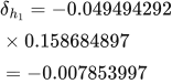 LaTeX:
\delta_{h_1} = -0.049494292 \times 0.158684897 = -0.007853997Step 5 input weights. Multiply the hidden delta by the corresponding raw input, not by the hidden output.
x1 → h1:
The sending value and receiving delta have different roles. All deltas still use the original forward-pass weights.
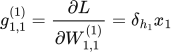
The receiving neuron supplies the delta; the sending neuron supplies the input value.
 LaTeX:
g_{1,1}^{(1)}=\frac{\partial L}{\partial W^{(1)}_{1,1}}=\delta_{h_1}x_1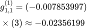 LaTeX:
g_{1,1}^{(1)}=(-0.007853997)\times(3)\approx -0.02356199Requested answers: dL/dw₂ = −0.066172539; dL/db₂ = −0.082490487. Negative gradients mean ordinary gradient descent would increase those parameters.