F25 Q5b

Answer — step by step

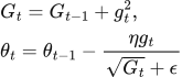
AdaGrad gives each parameter its own effective learning rate based on the sum of its past squared gradients. Start G₀ = 0, choose η and a small positive ε, then apply elementwise:

LaTeX: G_t=G_{t-1}+g_t^2,\quad\theta_t=\theta_{t-1}-\frac{\eta g_t}{\sqrt{G_t}+\epsilon}

Frequently updated coordinates accumulate a larger G and take smaller steps. Rarely active coordinates keep a relatively larger effective learning rate, which can be useful for sparse features. The square removes the sign in the accumulator; the unsquared current gradient still determines the direction of the parameter change.

Example with θ₀ = 1, η = 0.1, gradients 2 then 1 and negligible ε: first G = 4, denominator = 2, change = 0.1 × 2/2 = 0.1, θ₁ = 0.9. Next G = 5, denominator = √5 = 2.236068, change = 0.1/2.236068 = 0.04472136, θ₂ = 0.85527864.

Advantages over ordinary SGD include coordinatewise adaptation and usefulness for sparse gradients. Disadvantages include extra accumulator memory and continuously shrinking effective learning rates: G never decreases, so learning may become too slow. AdaGrad still requires a base learning rate and does not guarantee a global minimum. RMSProp addresses indefinite accumulation by replacing the sum with an exponentially weighted average.