Deep Learning · TEE · section
F25 Q6a
Final examination December 2025 fully solved
Question
Question (10 marks). Calculate every activation shape and trainable-parameter count for: Input 128 × 128 × 3. → Conv K = 3, filters = 16, stride = 1, padding = 0. → Pool K = 2, stride = 2, padding = 0. → Conv K = 3, filters = 32, stride = 1, padding = 0. → Pool K = 2, stride = 2, padding = 0. → Flatten. → Dense 240 units. → Dense 120 units. → Dense 5 units. Also convolve the input A with the kernel K shown below, valid padding and stride 2.
| 3 | 1 | 2 | 2 | 1 |
| 2 | 1 | 2 | 1 | 0 |
| 3 | 2 | 1 | 0 | 1 |
| 0 | 3 | 0 | 1 | 2 |
| 1 | 1 | 0 | 2 | 3 |
| 1 | 0 | −1 |
| 2 | 0 | −2 |
| 1 | 0 | −1 |
Stride 2; P = 0 (no padding).
Answer — step by step
Given
Input 128 × 128 × 3.
Conv K = 3, filters = 16, stride = 1, padding = 0.
Pool K = 2, stride = 2, padding = 0.
Conv K = 3, filters = 32, stride = 1, padding = 0.
Pool K = 2, stride = 2, padding = 0.
Dense 240 units.
Dense 120 units.
Dense 5 units.
Also convolve the input A with the kernel K shown below, valid padding and stride 2.
To find
Find every layer shape, its parameter count and the network total. Find every convolution output cell.
Formula — which one and why
Complete CNN calculation. Carry each output shape into the next layer. Convolution changes spatial size and channel count; pooling changes spatial size; flattening converts all activations into dense-layer inputs.
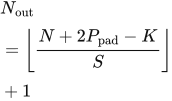
H,W,C = feature-map height, width and channels; K = kernel size; S = stride; P_pad = padding. One bias is assumed for each learned filter or dense neuron unless specified otherwise.
 LaTeX:
N_{\mathrm{out}}=\left\lfloor\frac{N+2P_{\mathrm{pad}}-K}{S}\right\rfloor+1 LaTeX:
P_{\mathrm{conv}}=(K^2C_{\mathrm{in}}+1)C_{\mathrm{out}} LaTeX:
n_{\mathrm{flat}}=HWC LaTeX:
P_{\mathrm{dense}}=(n_{\mathrm{in}}+1)n_{\mathrm{out}} LaTeX:
P_{\mathrm{pool}}=P_{\mathrm{flatten}}=0Yaad rakhne ka cue: Ek layer ka output, next layer ka input; shape aur parameters alag count.
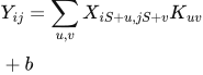
Convolution values. At each valid location, multiply corresponding window and kernel entries, add all products and add the filter bias once. Move by the stated stride and repeat.
X = input; K = kernel; S = stride; b = filter bias; u,v locate a kernel entry. Use the printed kernel without flipping under the stated deep-learning convention.
 LaTeX:
Y_{ij}=\sum_{u,v}X_{iS+u,jS+v}K_{uv}+bYaad rakhne ka cue: Matching cells multiply; sab products add; bias sirf ek baar.
Solution — step by step
Follow each selected input window below. Matching row colors connect its input cells, kernel coefficients and products; the outlined output cell shows where their sum belongs.
Use output size 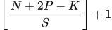 LaTeX:
\left\lfloor\frac{N+2P-K}{S}\right\rfloor+1, Conv weights K² × Cin × Cout and biases Cout, Dense weights Nin × Nout and biases Nout. Assume a bias per learned filter/unit, full input-channel connectivity and no trainable pooling parameters. ReLU and softmax activations themselves add no trainable parameters.
Layer-by-layer calculation
Carry the complete output shape of one layer into the next. Spatial size determines the number of activations; it does not multiply the number of shared convolution parameters.
Layer 1 — convolution
Spatial positions share the filter weights. Output depth equals the number of filters.
Input: 128 × 128 × 3. Use 16 filters of spatial size 3 × 3, stride 1, and padding 0 on each side.
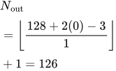
1. Calculate height and width.
 LaTeX:
N_{\mathrm{out}}=\left\lfloor\frac{128+2(0)-3}{1}\right\rfloor+1=1262. Determine output channels. Each filter produces one feature map. Therefore the output is 126 × 126 × 16.
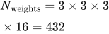
3. Count trainable values. Each filter receives all 3 input channels. Its weights are reused at every spatial position.
 LaTeX:
N_{\mathrm{weights}}=3\times3\times3\times16=432 LaTeX:
N_{\mathrm{biases}}=16 LaTeX:
P_1=432+16=448Layer 2 — pooling
Spatial dimensions change; the channel count stays the same. Pooling learns no weights.
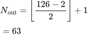
Input: 126 × 126 × 16. Use a 2 × 2 window, stride 2, and zero padding.
 LaTeX:
N_{\mathrm{out}}=\left\lfloor\frac{126-2}{2}\right\rfloor+1=63Pooling acts independently on each channel. The output is 63 × 63 × 16.
Trainable parameters: 0. Max/average pooling has no learned filter weights or biases.
Layer 3 — convolution
Spatial positions share the filter weights. Output depth equals the number of filters.
Input: 63 × 63 × 16. Use 32 filters of spatial size 3 × 3, stride 1, and padding 0 on each side.
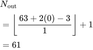
1. Calculate height and width.
 LaTeX:
N_{\mathrm{out}}=\left\lfloor\frac{63+2(0)-3}{1}\right\rfloor+1=612. Determine output channels. Each filter produces one feature map. Therefore the output is 61 × 61 × 32.
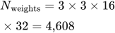
3. Count trainable values. Each filter receives all 16 input channels. Its weights are reused at every spatial position.
 LaTeX:
N_{\mathrm{weights}}=3\times3\times16\times32=4{,}608 LaTeX:
N_{\mathrm{biases}}=32 LaTeX:
P_3=4{,}608+32=4{,}640Layer 4 — pooling
Spatial dimensions change; the channel count stays the same. Pooling learns no weights.
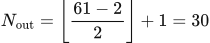
Input: 61 × 61 × 32. Use a 2 × 2 window, stride 2, and zero padding.
 LaTeX:
N_{\mathrm{out}}=\left\lfloor\frac{61-2}{2}\right\rfloor+1=30Pooling acts independently on each channel. The output is 30 × 30 × 32.
Trainable parameters: 0. Max/average pooling has no learned filter weights or biases.
The division gives 29.5; take its floor before adding 1. A partial window outside the unpadded input is not included.
Layer 5 — flatten
The same activation values are rearranged into one vector. No parameter is learned.
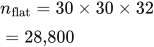
Input: 30 × 30 × 32. Rearrange all activation values into one vector.
 LaTeX:
n_{\mathrm{flat}}=30\times30\times32=28{,}800Output: a vector with 28,800 entries. Flattening changes the arrangement, so it adds 0 trainable parameters.
Layer 6 — fully connected layer
Every output neuron receives every input feature, with one bias per output neuron.
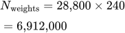
Input: 28,800 features. Output: 240 neurons. Every output neuron connects to every input feature and has one bias.
 LaTeX:
N_{\mathrm{weights}}=28{,}800\times240=6{,}912{,}000 LaTeX:
N_{\mathrm{biases}}=240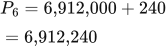 LaTeX:
P_6=6{,}912{,}000+240=6{,}912{,}240Layer 7 — fully connected layer
Every output neuron receives every input feature, with one bias per output neuron.
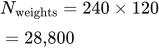
Input: 240 features. Output: 120 neurons. Every output neuron connects to every input feature and has one bias.
 LaTeX:
N_{\mathrm{weights}}=240\times120=28{,}800 LaTeX:
N_{\mathrm{biases}}=120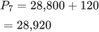 LaTeX:
P_7=28{,}800+120=28{,}920Layer 8 — fully connected layer
Every output neuron receives every input feature, with one bias per output neuron.
Input: 120 features. Output: 5 neurons. Every output neuron connects to every input feature and has one bias.
 LaTeX:
N_{\mathrm{weights}}=120\times5=600 LaTeX:
N_{\mathrm{biases}}=5 LaTeX:
P_8=600+5=605Summary of the complete network
| Layer | Spatial or flatten calculation | Output | Weights | Biases | Total |
|---|---|---|---|---|---|
| 1 conv | 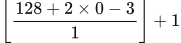 LaTeX: \left\lfloor\frac{128+2 \times 0-3}{1}\right\rfloor+1 | 126 x 126 x 16 | 432 | 16 | 448 |
| 2 pool | 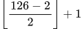 LaTeX: \left\lfloor\frac{126-2}{2}\right\rfloor+1 | 63 x 63 x 16 | 0 | 0 | 0 |
| 3 conv | 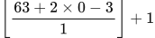 LaTeX: \left\lfloor\frac{63+2 \times 0-3}{1}\right\rfloor+1 | 61 x 61 x 32 | 4,608 | 32 | 4,640 |
| 4 pool | 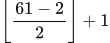 LaTeX: \left\lfloor\frac{61-2}{2}\right\rfloor+1 | 30 x 30 x 32 | 0 | 0 | 0 |
| 5 flat | 30 × 30 × 32 | 28800 | 0 | 0 | 0 |
| 6 dense | 28800 → 240 | 240 | 6,912,000 | 240 | 6,912,240 |
| 7 dense | 240 → 120 | 120 | 28,800 | 120 | 28,920 |
| 8 dense | 120 → 5 | 5 | 600 | 5 | 605 |
Parameter substitutions, in layer order:
Layer 1: (3 x 3 x 3 + 1) x 16 = 448.
Layer 3: (3 x 3 x 16 + 1) x 32 = 4,640.
Layer 6: (28800 + 1) x 240 = 6,912,240.
Layer 7: (240 + 1) x 120 = 28,920.
Layer 8: (120 + 1) x 5 = 605.
Total: 448 + 4,640 + 6,912,240 + 28,920 + 605 = 6,946,853 trainable parameters. Pooling changes activation size; it does not itself add learned weights. Always floor noninteger spatial dimensions.
Separate convolution calculation:
Step 1 shape: 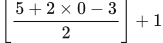 LaTeX:
\left\lfloor\frac{5+2 \times 0-3}{2}\right\rfloor+1 = 2 along each axis. Use the deep-learning cross-correlation convention: do not flip the printed kernel.
Output position (1, 1)
Use this position's input window. Multiply corresponding entries row by row; then add all row totals.
Input rows 1–3, columns 1–3. The window moves 2 cells per output step.
| 3 | 1 | 2 | 2 | 1 |
| 2 | 1 | 2 | 1 | 0 |
| 3 | 2 | 1 | 0 | 1 |
| 0 | 3 | 0 | 1 | 2 |
| 1 | 1 | 0 | 2 | 3 |
Only the outlined cells belong to this output.
| 1 | 0 | −1 |
| 2 | 0 | −2 |
| 1 | 0 | −1 |
Same row and column positions; no matrix multiplication.
| 3 | 0 | −2 |
| 4 | 0 | −4 |
| 3 | 0 | −1 |
Each cell is input × matching kernel coefficient.
1 + 0 + 2 = 3
| 3 | 5 |
| 3 | −7 |
Output row 1, column 1.
Window row 1.
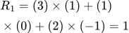 LaTeX:
R_1=(3)\times(1)+(1)\times(0)+(2)\times(-1)=1Window row 2.
 LaTeX:
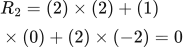
R_2=(2)\times(2)+(1)\times(0)+(2)\times(-2)=0Window row 3.
 LaTeX:
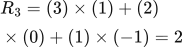
R_3=(3)\times(1)+(2)\times(0)+(1)\times(-1)=2Add the rows to obtain one output cell.
 LaTeX:
Y_{1,1}=(1)+(0)+(2)=3Output position (1, 2)
Use this position's input window. Multiply corresponding entries row by row; then add all row totals.
Input rows 1–3, columns 3–5. The window moves 2 cells per output step.
| 3 | 1 | 2 | 2 | 1 |
| 2 | 1 | 2 | 1 | 0 |
| 3 | 2 | 1 | 0 | 1 |
| 0 | 3 | 0 | 1 | 2 |
| 1 | 1 | 0 | 2 | 3 |
Only the outlined cells belong to this output.
| 1 | 0 | −1 |
| 2 | 0 | −2 |
| 1 | 0 | −1 |
Same row and column positions; no matrix multiplication.
| 2 | 0 | −1 |
| 4 | 0 | 0 |
| 1 | 0 | −1 |
Each cell is input × matching kernel coefficient.
1 + 4 + 0 = 5
| 3 | 5 |
| 3 | −7 |
Output row 1, column 2.
Window row 1.
 LaTeX:
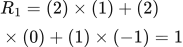
R_1=(2)\times(1)+(2)\times(0)+(1)\times(-1)=1Window row 2.
 LaTeX:
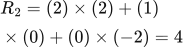
R_2=(2)\times(2)+(1)\times(0)+(0)\times(-2)=4Window row 3.
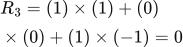 LaTeX:
R_3=(1)\times(1)+(0)\times(0)+(1)\times(-1)=0Add the rows to obtain one output cell.
 LaTeX:
Y_{1,2}=(1)+(4)+(0)=5Output position (2, 1)
Use this position's input window. Multiply corresponding entries row by row; then add all row totals.
Input rows 3–5, columns 1–3. The window moves 2 cells per output step.
| 3 | 1 | 2 | 2 | 1 |
| 2 | 1 | 2 | 1 | 0 |
| 3 | 2 | 1 | 0 | 1 |
| 0 | 3 | 0 | 1 | 2 |
| 1 | 1 | 0 | 2 | 3 |
Only the outlined cells belong to this output.
| 1 | 0 | −1 |
| 2 | 0 | −2 |
| 1 | 0 | −1 |
Same row and column positions; no matrix multiplication.
| 3 | 0 | −1 |
| 0 | 0 | 0 |
| 1 | 0 | 0 |
Each cell is input × matching kernel coefficient.
2 + 0 + 1 = 3
| 3 | 5 |
| 3 | −7 |
Output row 2, column 1.
Window row 1.
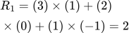 LaTeX:
R_1=(3)\times(1)+(2)\times(0)+(1)\times(-1)=2Window row 2.
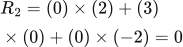 LaTeX:
R_2=(0)\times(2)+(3)\times(0)+(0)\times(-2)=0Window row 3.
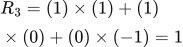 LaTeX:
R_3=(1)\times(1)+(1)\times(0)+(0)\times(-1)=1Add the rows to obtain one output cell.
 LaTeX:
Y_{2,1}=(2)+(0)+(1)=3Output position (2, 2)
Use this position's input window. Multiply corresponding entries row by row; then add all row totals.
Input rows 3–5, columns 3–5. The window moves 2 cells per output step.
| 3 | 1 | 2 | 2 | 1 |
| 2 | 1 | 2 | 1 | 0 |
| 3 | 2 | 1 | 0 | 1 |
| 0 | 3 | 0 | 1 | 2 |
| 1 | 1 | 0 | 2 | 3 |
Only the outlined cells belong to this output.
| 1 | 0 | −1 |
| 2 | 0 | −2 |
| 1 | 0 | −1 |
Same row and column positions; no matrix multiplication.
| 1 | 0 | −1 |
| 0 | 0 | −4 |
| 0 | 0 | −3 |
Each cell is input × matching kernel coefficient.
0 + (−4) + (−3) = −7
| 3 | 5 |
| 3 | −7 |
Output row 2, column 2.
Window row 1.
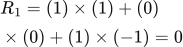 LaTeX:
R_1=(1)\times(1)+(0)\times(0)+(1)\times(-1)=0Window row 2.
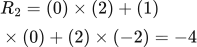 LaTeX:
R_2=(0)\times(2)+(1)\times(0)+(2)\times(-2)=-4Window row 3.
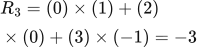 LaTeX:
R_3=(0)\times(1)+(2)\times(0)+(3)\times(-1)=-3Add the rows to obtain one output cell.
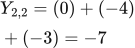 LaTeX:
Y_{2,2}=(0)+(-4)+(-3)=-7Final output:  LaTeX:
\begin{bmatrix}3 & 5\\3 & -7\end{bmatrix}. Each output came from its own complete window; stride changes the next window position, not the multiplication rule.