Deep Learning · TEE · section
R26 Q2a
Re examination February 2026 fully solved
Question
Question (10 marks). Use the sigmoid network Input x = [0.25, 0.7]. Each row below lists the incoming weights of one receiving neuron. W₁ is shown below; b₁ = [1, 1]; W₂ is shown below; b₂ = [1, 1]. Hidden and output activations are sigmoid. Target y = [0.7, 0.3]. Learning rate η = 1. Here w₁ = x₁ → h₁, w₅ = h₁ → o₁ and w₇ = h₁ → o₂. Run forward and backward passes and update w₁, w₅, w₇. The paper gives no explicit loss formula.
Answer — step by step
Given
Input x = [0.25,0.7]; W₁ and W₂ are printed with the question.
Hidden biases = [1,1]; output biases = [1,1]; all activations sigmoid.
Target = [0.7,0.3]; η = 1.
The paper omits the loss; this solution explicitly assumes half summed squared loss.
To find
Calculate forward values and update only w₁ = x₁→h₁, w₅ = h₁→o₁ and w₇ = h₁→o₂.
Formula — which one and why
Forward propagation. Evaluate one layer completely before supplying its activated outputs to the next layer. Each layer has its own weights and biases.
x = input vector; h = hidden outputs; W₁,b₁ = hidden parameters; W₂,b₂ = output parameters; f₁,f₂ = the stated activations.
 LaTeX:
z_h=W_1x+b_1 LaTeX:
h=f_1(z_h) LaTeX:
z_o=W_2h+b_2 LaTeX:
o=f_2(z_o)Yaad rakhne ka cue: Pehli layer ka activated output hi agli layer ka input hai.
Half summed squared loss. This loss convention takes one-half of the sum of squared prediction errors. Use it when the question specifies it, or explicitly state it as an assumption when the paper omits the loss. Differentiating cancels the factor one-half against the square derivative.
oⱼ = output j; yⱼ = target j; L = half summed squared loss under the stated or explicitly assumed convention.
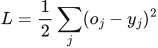 LaTeX:
L=\frac12\sum_j(o_j-y_j)^2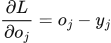 LaTeX:
\frac{\partial L}{\partial o_j}=o_j-y_jYaad rakhne ka cue: Half aur square ka 2 cancel: output derivative = prediction − target.
Sigmoid and its slope. Use sigmoid when the neuron is specified to squash its preactivation into (0,1). Once its output is known, its derivative needs only output × (1−output).
z = preactivation; p = sigmoid output; e is the exponential base, not a prediction error in this formula.
 LaTeX:
p=\frac{1}{1+e^{-z}}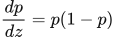 LaTeX:
\frac{dp}{dz}=p(1-p)Yaad rakhne ka cue: Sigmoid output p; uska slope p × (1−p).
Backpropagation. The loss tells us how each output must change. Multiply by that neuron’s activation slope to obtain its delta. A weight gradient is receiving delta × sending value. Hidden deltas must include every outgoing path.
δ (delta) = derivative of loss with respect to a neuron’s preactivation; f′ = activation derivative; aᵢ = sending activation; Wⱼᵢ = connection weight. Use the exact loss scaling in the question.
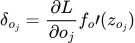 LaTeX:
\delta_{o_j}=\frac{\partial L}{\partial o_j}f_o\prime(z_{o_j})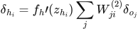 LaTeX:
\delta_{h_i}=f_h\prime(z_{h_i})\sum_jW_{ji}^{(2)}\delta_{o_j}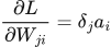 LaTeX:
\frac{\partial L}{\partial W_{ji}}=\delta_ja_i LaTeX:
\frac{\partial L}{\partial b_j}=\delta_j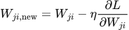 LaTeX:
W_{ji,\mathrm{new}}=W_{ji}-\eta\frac{\partial L}{\partial W_{ji}}Yaad rakhne ka cue: Receiving delta × sending value = us connection ka gradient.
Solution — step by step
Step 1 map the arrows. Each row of W₁ receives all inputs; each row of W₂ receives all hidden outputs. Bias is added once per receiving neuron. All gradients below use the OLD weights from this same forward pass.
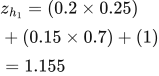
Hidden neuron 1:
 LaTeX:
z_{h_1} = (0.2 \times 0.25) + (0.15 \times 0.7) + (1) = 1.155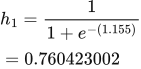 LaTeX:
h_{1}=\frac{1}{1+e^{-(1.155)}}=0.760423002Hidden neuron 2:
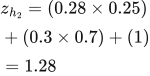 LaTeX:
z_{h_2} = (0.28 \times 0.25) + (0.3 \times 0.7) + (1) = 1.28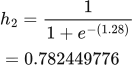 LaTeX:
h_{2}=\frac{1}{1+e^{-(1.28)}}=0.782449776Output neuron 1:
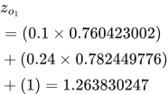 LaTeX:
z_{o_1} = (0.1 \times 0.760423002) + (0.24 \times 0.782449776) + (1) = 1.263830247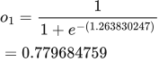 LaTeX:
o_{1}=\frac{1}{1+e^{-(1.263830247)}}=0.779684759Output neuron 2:
 LaTeX:
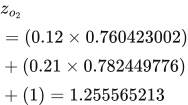
z_{o_2} = (0.12 \times 0.760423002) + (0.21 \times 0.782449776) + (1) = 1.255565213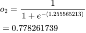 LaTeX:
o_{2}=\frac{1}{1+e^{-(1.255565213)}}=0.778261739Step 2 loss convention. This worked solution uses half summed squared loss, L = ½Σ(o − y)². Follow the loss specified in the question; where none is supplied, this is an explicit assumption.
Prediction minus target = [0.079684759, 0.478261739]. Squared errors = [0.006349661, 0.228734291]. Half-sum squared loss = 0.117541976; mean squared error = 0.117541976. These are different unless the number of output components makes the scale coincide.
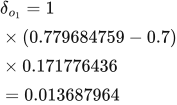
Output delta 1:
 LaTeX:
\delta_{o_1} = 1 \times (0.779684759-0.7) \times 0.171776436 = 0.013687964The derivative is o(1−o).
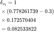
Output delta 2:
 LaTeX:
\delta_{o_2} = 1 \times (0.778261739-0.3) \times 0.172570404 = 0.082533822The derivative is o(1−o).
Step 3 output weights. Gradient = receiving delta × sending activation. An output bias gradient equals its delta.
h1 → o1:
Subtract η × gradient = 0.010408643. This weight decreases.
The sending value and receiving delta have different roles. All deltas still use the original forward-pass weights.
The receiving neuron supplies the delta; the sending neuron supplies its activation.
 LaTeX:
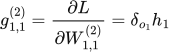
g_{1,1}^{(2)}=\frac{\partial L}{\partial W^{(2)}_{1,1}}=\delta_{o_1}h_1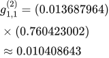 LaTeX:
g_{1,1}^{(2)}=(0.013687964)\times(0.760423002)\approx 0.010408643Apply the learning rate to this gradient and subtract the result from the old weight.
 LaTeX:
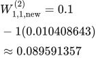
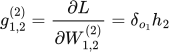
W^{(2)}_{1,1,\mathrm{new}}=0.1-1(0.010408643)\approx 0.089591357h2 → o1:
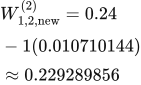
Subtract η × gradient = 0.010710144. This weight decreases.
The sending value and receiving delta have different roles. All deltas still use the original forward-pass weights.
The receiving neuron supplies the delta; the sending neuron supplies its activation.
 LaTeX:
g_{1,2}^{(2)}=\frac{\partial L}{\partial W^{(2)}_{1,2}}=\delta_{o_1}h_2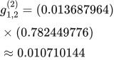 LaTeX:
g_{1,2}^{(2)}=(0.013687964)\times(0.782449776)\approx 0.010710144Apply the learning rate to this gradient and subtract the result from the old weight.
 LaTeX:
W^{(2)}_{1,2,\mathrm{new}}=0.24-1(0.010710144)\approx 0.229289856h1 → o2:
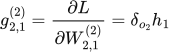
Subtract η × gradient = 0.062760617. This weight decreases.
The sending value and receiving delta have different roles. All deltas still use the original forward-pass weights.
The receiving neuron supplies the delta; the sending neuron supplies its activation.
 LaTeX:
g_{2,1}^{(2)}=\frac{\partial L}{\partial W^{(2)}_{2,1}}=\delta_{o_2}h_1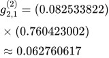 LaTeX:
g_{2,1}^{(2)}=(0.082533822)\times(0.760423002)\approx 0.062760617Apply the learning rate to this gradient and subtract the result from the old weight.
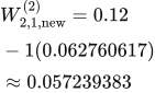 LaTeX:
W^{(2)}_{2,1,\mathrm{new}}=0.12-1(0.062760617)\approx 0.057239383h2 → o2:
Subtract η × gradient = 0.06457857. This weight decreases.
The sending value and receiving delta have different roles. All deltas still use the original forward-pass weights.
The receiving neuron supplies the delta; the sending neuron supplies its activation.
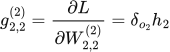 LaTeX:
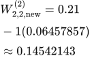
g_{2,2}^{(2)}=\frac{\partial L}{\partial W^{(2)}_{2,2}}=\delta_{o_2}h_2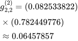 LaTeX:
g_{2,2}^{(2)}=(0.082533822)\times(0.782449776)\approx 0.06457857Apply the learning rate to this gradient and subtract the result from the old weight.
 LaTeX:
W^{(2)}_{2,2,\mathrm{new}}=0.21-1(0.06457857)\approx 0.14542143Step 4 hidden deltas. A hidden unit can influence EVERY connected output, so add those paths BEFORE multiplying by the hidden activation derivative.
Hidden 1 downstream contribution:
Calculate each outgoing path using the old outgoing weight and that output's delta.
Multiply within each path. Add the resulting contributions at the shared hidden neuron.
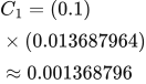
Contribution from output 1.
 LaTeX:
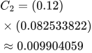
C_1=(0.1)\times(0.013687964)\approx 0.001368796Contribution from output 2.
 LaTeX:
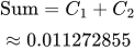
C_2=(0.12)\times(0.082533822)\approx 0.009904059Accumulate the contributions, then apply the hidden activation derivative below.
 LaTeX:
\text{Sum}=C_1+C_2\approx 0.011272855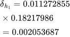 LaTeX:
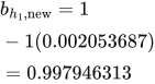
\delta_{h_1} = 0.011272855 \times 0.18217986 = 0.002053687Hidden 2 downstream contribution:
Calculate each outgoing path using the old outgoing weight and that output's delta.
Multiply within each path. Add the resulting contributions at the shared hidden neuron.
Contribution from output 1.
 LaTeX:
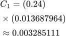
C_1=(0.24)\times(0.013687964)\approx 0.003285111Contribution from output 2.
 LaTeX:
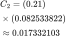
C_2=(0.21)\times(0.082533822)\approx 0.017332103Accumulate the contributions, then apply the hidden activation derivative below.
 LaTeX:
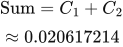
\text{Sum}=C_1+C_2\approx 0.020617214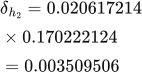 LaTeX:
\delta_{h_2} = 0.020617214 \times 0.170222124 = 0.003509506Step 5 input weights. Multiply the hidden delta by the corresponding raw input, not by the hidden output.
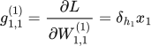
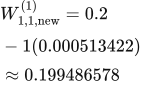
x1 → h1:
Subtract η × gradient = 0.000513422. This weight decreases.
The sending value and receiving delta have different roles. All deltas still use the original forward-pass weights.
The receiving neuron supplies the delta; the sending neuron supplies the input value.
 LaTeX:
g_{1,1}^{(1)}=\frac{\partial L}{\partial W^{(1)}_{1,1}}=\delta_{h_1}x_1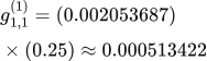 LaTeX:
g_{1,1}^{(1)}=(0.002053687)\times(0.25)\approx 0.000513422Apply the learning rate to this gradient and subtract the result from the old weight.
 LaTeX:
W^{(1)}_{1,1,\mathrm{new}}=0.2-1(0.000513422)\approx 0.199486578x2 → h1:
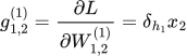
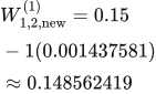
Subtract η × gradient = 0.001437581. This weight decreases.
The sending value and receiving delta have different roles. All deltas still use the original forward-pass weights.
The receiving neuron supplies the delta; the sending neuron supplies the input value.
 LaTeX:
g_{1,2}^{(1)}=\frac{\partial L}{\partial W^{(1)}_{1,2}}=\delta_{h_1}x_2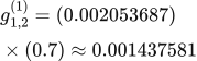 LaTeX:
g_{1,2}^{(1)}=(0.002053687)\times(0.7)\approx 0.001437581Apply the learning rate to this gradient and subtract the result from the old weight.
 LaTeX:
W^{(1)}_{1,2,\mathrm{new}}=0.15-1(0.001437581)\approx 0.148562419x1 → h2:
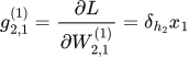
Subtract η × gradient = 0.000877376. This weight decreases.
The sending value and receiving delta have different roles. All deltas still use the original forward-pass weights.
The receiving neuron supplies the delta; the sending neuron supplies the input value.
 LaTeX:
g_{2,1}^{(1)}=\frac{\partial L}{\partial W^{(1)}_{2,1}}=\delta_{h_2}x_1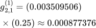 LaTeX:
g_{2,1}^{(1)}=(0.003509506)\times(0.25)\approx 0.000877376Apply the learning rate to this gradient and subtract the result from the old weight.
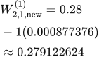 LaTeX:
W^{(1)}_{2,1,\mathrm{new}}=0.28-1(0.000877376)\approx 0.279122624x2 → h2:
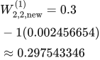
Subtract η × gradient = 0.002456654. This weight decreases.
The sending value and receiving delta have different roles. All deltas still use the original forward-pass weights.
The receiving neuron supplies the delta; the sending neuron supplies the input value.
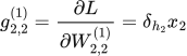 LaTeX:
g_{2,2}^{(1)}=\frac{\partial L}{\partial W^{(1)}_{2,2}}=\delta_{h_2}x_2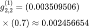 LaTeX:
g_{2,2}^{(1)}=(0.003509506)\times(0.7)\approx 0.002456654Apply the learning rate to this gradient and subtract the result from the old weight.
 LaTeX:
W^{(1)}_{2,2,\mathrm{new}}=0.3-1(0.002456654)\approx 0.297543346Step 6 bias updates. A bias receives a constant input 1, so its gradient equals the corresponding delta. Use the same old forward pass and learning rate as the weight updates.
 LaTeX:
b_{h_1,\mathrm{new}}=1-1(0.002053687)=0.997946313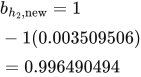 LaTeX:
b_{h_2,\mathrm{new}}=1-1(0.003509506)=0.996490494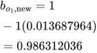 LaTeX:
b_{o_1,\mathrm{new}}=1-1(0.013687964)=0.986312036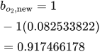 LaTeX:
b_{o_2,\mathrm{new}}=1-1(0.082533822)=0.917466178These are independent per-neuron biases. If the question fixes biases, keep them fixed. If it specifies a single tied bias, add all deltas sharing that bias before updating it.
Requested updates: w₁ = 0.199486578, w₅ = 0.089591357, w₇ = 0.057239383. For two outputs, this chosen half-sum equals their MSE; an unaveraged unhalved sum would double the gradients.