Deep Learning · TEE · section
R26 Q4a
Re examination February 2026 fully solved
Question
Question (10 marks). Compare batch GD and SGD for loss oscillations with a graph, memory and large datasets. Discuss learning rate extremes. For J(θ) = 0.7 θ³, θ₀ = 1, η = 0.1, perform two iterations.
Answer — step by step
Given
J(θ) = 0.7θ³; θ₀ = 1; η = 0.1.
To find
Calculate the derivative and perform two updates.
Formula — which one and why
Gradient descent. Evaluate the gradient at the current parameter, multiply by the learning rate and subtract. If the objective is supplied, differentiate it and recompute the gradient after each update.
θ (theta) = trainable parameter; g = derivative of the stated objective J; η = learning rate; t labels the update number.
 LaTeX:
g_t=J\prime(\theta_{t-1}) LaTeX:
\theta_t=\theta_{t-1}-\eta g_tYaad rakhne ka cue: Naya = purana − learning rate × current gradient.
Solution — step by step
The learning rate η determines update size: θ new = θ old − ηg. A rate that is too small can make progress extremely slow; one that is too large can overshoot, oscillate or diverge. Nonconvex objectives can contain flat regions, saddle points and local minima. Poor scaling can cause long zig-zag paths; vanishing or exploding gradients can make training ineffective or unstable.
Batch gradient descent uses all N samples per update, SGD uses one sample, and mini-batch uses B samples. Batch updates are less noisy for a fixed dataset but costly; SGD makes frequent noisy updates; mini-batches balance vectorized computation and stochasticity. Data need not all reside in memory even for a full gradient because gradients can be accumulated, but larger simultaneous batches require more activation memory.
Momentum accumulates a running direction, helping movement persist across consistent gradients and damping some oscillation. Mini-batching describes which data forms a gradient; momentum describes how that gradient is used. They can be combined, so they are not competing categories.
Diagnose stalled training by checking data, preprocessing, losses and gradients before blindly adding layers. Compare training and validation curves, tune learning rate, inspect saturation and use appropriate initialization or adaptive optimization. A noisy curve with a decreasing trend can be normal for SGD.
Step 1: differentiate the objective before substituting.
 LaTeX:
J(\theta)=0.7\theta^3 LaTeX:
g(\theta)=0.7(3)\theta^2=2.1\theta^2Step 2: evaluate gradient at the original parameter.
 LaTeX:
g_1=2.1(1)^2=2.1Step 3: scale the first gradient.
 LaTeX:
0.1(2.1)=0.21Step 4: subtract to obtain the first update.
 LaTeX:
\theta_1=1-0.21=0.79Step 5: square the changed parameter.
 LaTeX:
0.79^2=0.6241Step 6: recalculate the gradient.
 LaTeX:
g_2=2.1(0.6241)=1.31061Step 7: scale the second gradient.
 LaTeX:
0.1(1.31061)=0.131061Step 8: subtract from the first updated parameter.
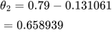 LaTeX:
\theta_2=0.79-0.131061=0.658939Final answer: θ₁ = 0.79; θ₂ = 0.658939. No individual samples are supplied, so these are the stated scalar gradient updates. The cubic is unbounded below; two steps are not a convergence proof.