Deep Learning · TEE · section
F23 Q1c
Final examination December 2023 fully solved
Question
Question (5 marks). Draw a time-unrolled RNN and briefly explain training by backpropagation through time.
Answer — step by step
Backpropagation through time trains an RNN by treating its time-unrolled computations as a deep computational graph.
1. Initialize the hidden state and run the forward recurrence from the first input to the last.
2. Compute the specified output loss, at the final step or across several steps.
3. Start from the last loss and propagate derivatives backwards through output and hidden operations.
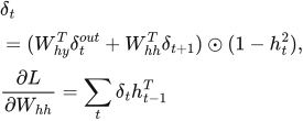
4. At each earlier state, add the direct output-loss contribution and the contribution arriving from future states.
5. Sum all uses of each shared weight before applying the optimizer update.
 LaTeX:
\delta_t=(W_{hy}^{T}\delta_t^{out}+W_{hh}^{T}\delta_{t+1})\odot(1-h_t^2),\quad \frac{\partial L}{\partial W_{hh}}=\sum_t\delta_t h_{t-1}^{T}The tanh derivative is 1−h². Repeated multiplication by recurrent weights and activation derivatives may shrink gradients toward zero or amplify them greatly. Early words then receive a weak learning signal or updates become unstable. Gated architectures help long-context learning; suitable initialization and learning rates help training; clipping limits exploding gradients. Truncated BPTT restricts the backward time window to reduce computation and memory. It does not mean creating independent weights for each time step.