Deep Learning · TEE · section
F22 Q1a
Final examination November 2022 fully solved
Question
Question (4 marks). A normalized 5 × 5 image has every row [0.5,0.5,0.3,0.3,0.3]. Convolve it with a 3 × 3 filter whose every row is [1,0,−1], stride 2, no padding. Compute the output and identify the feature.
Answer — step by step
Given
A normalized 5 × 5 image has every row [0.5,0.5,0.3,0.3,0.3].
Convolve it with a 3 × 3 filter whose every row is [1,0,−1], stride 2, no padding.
To find
Find every convolution output cell.
Formula — which one and why
Convolution values. At each valid location, multiply corresponding window and kernel entries, add all products and add the filter bias once. Move by the stated stride and repeat.
X = input; K = kernel; S = stride; b = filter bias; u,v locate a kernel entry. Use the printed kernel without flipping under the stated deep-learning convention.
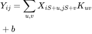 LaTeX:
Y_{ij}=\sum_{u,v}X_{iS+u,jS+v}K_{uv}+bYaad rakhne ka cue: Matching cells multiply; sab products add; bias sirf ek baar.
Solution — step by step
Follow each selected input window below. Matching row colors connect its input cells, kernel coefficients and products; the outlined output cell shows where their sum belongs.
Step 1 shape: 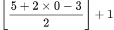 LaTeX:
\left\lfloor\frac{5+2 \times 0-3}{2}\right\rfloor+1 = 2 along each axis. Use the deep-learning cross-correlation convention: do not flip the printed kernel.
Output position (1, 1)
Use this position's input window. Multiply corresponding entries row by row; then add all row totals.
Input rows 1–3, columns 1–3. The window moves 2 cells per output step.
| 0.5 | 0.5 | 0.3 | 0.3 | 0.3 |
| 0.5 | 0.5 | 0.3 | 0.3 | 0.3 |
| 0.5 | 0.5 | 0.3 | 0.3 | 0.3 |
| 0.5 | 0.5 | 0.3 | 0.3 | 0.3 |
| 0.5 | 0.5 | 0.3 | 0.3 | 0.3 |
Only the outlined cells belong to this output.
| 1 | 0 | −1 |
| 1 | 0 | −1 |
| 1 | 0 | −1 |
Same row and column positions; no matrix multiplication.
| 0.5 | 0 | −0.3 |
| 0.5 | 0 | −0.3 |
| 0.5 | 0 | −0.3 |
Each cell is input × matching kernel coefficient.
0.2 + 0.2 + 0.2 = 0.6
| 0.6 | 0 |
| 0.6 | 0 |
Output row 1, column 1.
Window row 1.
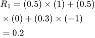 LaTeX:
R_1=(0.5)\times(1)+(0.5)\times(0)+(0.3)\times(-1)=0.2Window row 2.
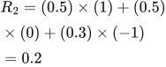 LaTeX:
R_2=(0.5)\times(1)+(0.5)\times(0)+(0.3)\times(-1)=0.2Window row 3.
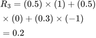 LaTeX:
R_3=(0.5)\times(1)+(0.5)\times(0)+(0.3)\times(-1)=0.2Add the rows to obtain one output cell.
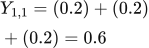 LaTeX:
Y_{1,1}=(0.2)+(0.2)+(0.2)=0.6Output position (1, 2)
Use this position's input window. Multiply corresponding entries row by row; then add all row totals.
Input rows 1–3, columns 3–5. The window moves 2 cells per output step.
| 0.5 | 0.5 | 0.3 | 0.3 | 0.3 |
| 0.5 | 0.5 | 0.3 | 0.3 | 0.3 |
| 0.5 | 0.5 | 0.3 | 0.3 | 0.3 |
| 0.5 | 0.5 | 0.3 | 0.3 | 0.3 |
| 0.5 | 0.5 | 0.3 | 0.3 | 0.3 |
Only the outlined cells belong to this output.
| 1 | 0 | −1 |
| 1 | 0 | −1 |
| 1 | 0 | −1 |
Same row and column positions; no matrix multiplication.
| 0.3 | 0 | −0.3 |
| 0.3 | 0 | −0.3 |
| 0.3 | 0 | −0.3 |
Each cell is input × matching kernel coefficient.
0 + 0 + 0 = 0
| 0.6 | 0 |
| 0.6 | 0 |
Output row 1, column 2.
Window row 1.
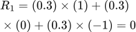 LaTeX:
R_1=(0.3)\times(1)+(0.3)\times(0)+(0.3)\times(-1)=0Window row 2.
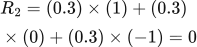 LaTeX:
R_2=(0.3)\times(1)+(0.3)\times(0)+(0.3)\times(-1)=0Window row 3.
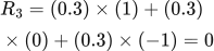 LaTeX:
R_3=(0.3)\times(1)+(0.3)\times(0)+(0.3)\times(-1)=0Add the rows to obtain one output cell.
 LaTeX:
Y_{1,2}=(0)+(0)+(0)=0Output position (2, 1)
Use this position's input window. Multiply corresponding entries row by row; then add all row totals.
Input rows 3–5, columns 1–3. The window moves 2 cells per output step.
| 0.5 | 0.5 | 0.3 | 0.3 | 0.3 |
| 0.5 | 0.5 | 0.3 | 0.3 | 0.3 |
| 0.5 | 0.5 | 0.3 | 0.3 | 0.3 |
| 0.5 | 0.5 | 0.3 | 0.3 | 0.3 |
| 0.5 | 0.5 | 0.3 | 0.3 | 0.3 |
Only the outlined cells belong to this output.
| 1 | 0 | −1 |
| 1 | 0 | −1 |
| 1 | 0 | −1 |
Same row and column positions; no matrix multiplication.
| 0.5 | 0 | −0.3 |
| 0.5 | 0 | −0.3 |
| 0.5 | 0 | −0.3 |
Each cell is input × matching kernel coefficient.
0.2 + 0.2 + 0.2 = 0.6
| 0.6 | 0 |
| 0.6 | 0 |
Output row 2, column 1.
Window row 1.
LaTeX: R_1=(0.5)\times(1)+(0.5)\times(0)+(0.3)\times(-1)=0.2Window row 2.
LaTeX: R_2=(0.5)\times(1)+(0.5)\times(0)+(0.3)\times(-1)=0.2Window row 3.
LaTeX: R_3=(0.5)\times(1)+(0.5)\times(0)+(0.3)\times(-1)=0.2Add the rows to obtain one output cell.
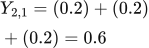 LaTeX:
Y_{2,1}=(0.2)+(0.2)+(0.2)=0.6Output position (2, 2)
Use this position's input window. Multiply corresponding entries row by row; then add all row totals.
Input rows 3–5, columns 3–5. The window moves 2 cells per output step.
| 0.5 | 0.5 | 0.3 | 0.3 | 0.3 |
| 0.5 | 0.5 | 0.3 | 0.3 | 0.3 |
| 0.5 | 0.5 | 0.3 | 0.3 | 0.3 |
| 0.5 | 0.5 | 0.3 | 0.3 | 0.3 |
| 0.5 | 0.5 | 0.3 | 0.3 | 0.3 |
Only the outlined cells belong to this output.
| 1 | 0 | −1 |
| 1 | 0 | −1 |
| 1 | 0 | −1 |
Same row and column positions; no matrix multiplication.
| 0.3 | 0 | −0.3 |
| 0.3 | 0 | −0.3 |
| 0.3 | 0 | −0.3 |
Each cell is input × matching kernel coefficient.
0 + 0 + 0 = 0
| 0.6 | 0 |
| 0.6 | 0 |
Output row 2, column 2.
Window row 1.
LaTeX: R_1=(0.3)\times(1)+(0.3)\times(0)+(0.3)\times(-1)=0Window row 2.
LaTeX: R_2=(0.3)\times(1)+(0.3)\times(0)+(0.3)\times(-1)=0Window row 3.
LaTeX: R_3=(0.3)\times(1)+(0.3)\times(0)+(0.3)\times(-1)=0Add the rows to obtain one output cell.
 LaTeX:
Y_{2,2}=(0)+(0)+(0)=0Final output:  LaTeX:
\begin{bmatrix}0.6 & 0\\0.6 & 0\end{bmatrix}. Each output came from its own complete window; stride changes the next window position, not the multiplication rule.
The filter compares left and right neighborhoods and responds to a vertical brightness boundary. Inputs are already normalized. No additional output-normalization rule is supplied, so the determined convolution is LaTeX: \begin{bmatrix}0.6 & 0\\0.6 & 0\end{bmatrix}. If an examiner explicitly requests min-max normalization of this result, divide by 0.6 to obtain  LaTeX:
\begin{bmatrix}1 & 0\\1 & 0\end{bmatrix}; that is a separate stated operation.