F22 Q4b

Answer — step by step

Given

6 inputs → hidden 5 → hidden 5 → 4 output classes.

AdaGrad is the specified training algorithm; one bias per receiving neuron.

To find

Draw the architecture and count its learned weights/biases. The optimizer name does not change the count.

Formula — which one and why

Dense-layer parameters. Every output neuron receives every input, so multiply inputs by outputs for weights. Add one bias per receiving neuron. Sum separate layers.

n_in = incoming features; n_out = receiving neurons. The input layer itself has no learned receiving weights or biases.

LaTeX: P=(n_{\mathrm{in}}+1)n_{\mathrm{out}}

Yaad rakhne ka cue: Har output ke liye saare inputs plus ek bias.

Solution — step by step

Architecture: 6 → 5 → 5 → 4. Each non-input neuron has one bias.

Diagram: F22 Q4b the input has six features and the output has four classes. Labels: Input | 6 neurons | Hidden 1 | 5 neurons | Hidden 2 | 5 neurons | Output | 4 neurons | Every receiving neuron has one bias. All adjacent layers are fully connected.

Layer 6 → 5

Step 1: count connections.

LaTeX: 6(5)=30

Step 2: count receiving-neuron biases.

There are 5 receiving neurons, so 5 biases.

Step 3: add weights and biases.

LaTeX: 30+5=35

Layer 5 → 5

Step 1: count connections.

LaTeX: 5(5)=25

Step 2: count receiving-neuron biases.

There are 5 receiving neurons, so 5 biases.

Step 3: add weights and biases.

LaTeX: 25+5=30

Layer 5 → 4

Step 1: count connections.

LaTeX: 5(4)=20

Step 2: count receiving-neuron biases.

There are 4 receiving neurons, so 4 biases.

Step 3: add weights and biases.

LaTeX: 20+4=24

Total = 89. Input values and activations are not trainable parameters.

The learned parameters are input-to-hidden, hidden-to-hidden and hidden-to-output weights plus biases at receiving neurons. AdaGrad accumulators are optimizer state, not additional predictive weights. Hyperparameters include hidden widths/depth, learning rate η,ε, batch size, epochs, activations and regularization settings. Use 4-class softmax with categorical cross-entropy.

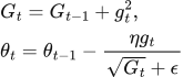
AdaGrad gives each parameter its own effective learning rate based on the sum of its past squared gradients. Start G₀ = 0, choose η and a small positive ε, then apply elementwise:

LaTeX: G_t=G_{t-1}+g_t^2,\quad\theta_t=\theta_{t-1}-\frac{\eta g_t}{\sqrt{G_t}+\epsilon}

Frequently updated coordinates accumulate a larger G and take smaller steps. Rarely active coordinates keep a relatively larger effective learning rate, which can be useful for sparse features. The square removes the sign in the accumulator; the unsquared current gradient still determines the direction of the parameter change.

Example with θ₀ = 1, η = 0.1, gradients 2 then 1 and negligible ε: first G = 4, denominator = 2, change = 0.1 × 2/2 = 0.1, θ₁ = 0.9. Next G = 5, denominator = √5 = 2.236068, change = 0.1/2.236068 = 0.04472136, θ₂ = 0.85527864.

Advantages over ordinary SGD include coordinatewise adaptation and usefulness for sparse gradients. Disadvantages include extra accumulator memory and continuously shrinking effective learning rates: G never decreases, so learning may become too slow. AdaGrad still requires a base learning rate and does not guarantee a global minimum. RMSProp addresses indefinite accumulation by replacing the sum with an exponentially weighted average.