Deep Learning · TEE · section
F22 Q5a
Final examination November 2022 fully solved
Question
Question (10 marks). Develop an RNN with hidden states and explain gradient updates using backpropagation.
Answer — step by step
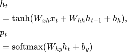
A recurrent neural network processes a sequence in order and maintains a hidden state that summarizes earlier information. Its weights are shared across time steps.
 LaTeX:
h_t=\tanh(W_{xh}x_t+W_{hh}h_{t-1}+b_h),\quad p_t=\operatorname{softmax}(W_{hy}h_t+b_y)At each step, transform the current token representation, transform the previous hidden state, add the bias and apply the activation. An output layer may produce a prediction at each step or only at the end. This allows a sequence's length to vary while the parameter set stays fixed.
For next-word prediction, tokenize text, represent each word numerically, update the state for each prefix token, and apply an output softmax over the vocabulary. Train against the actual next token using cross-entropy. For sentiment classification, use the sequence representation to predict positive, neutral or negative. Word order matters: “not good” should not be interpreted like “good”.
A basic feedforward model has no built-in recurrent state, though a fixed window can be supplied explicitly. RNNs provide recurrent context but have sequential computation costs and difficulty learning long dependencies because of vanishing or exploding gradients. An encoder-decoder RNN can encode a source sentence and generate a target sentence of a different length; this is a historical RNN translation explanation, not a claim about any commercial service's current architecture.
Backpropagation through time trains an RNN by treating its time-unrolled computations as a deep computational graph.
1. Initialize the hidden state and run the forward recurrence from the first input to the last.
2. Compute the specified output loss, at the final step or across several steps.
3. Start from the last loss and propagate derivatives backwards through output and hidden operations.
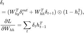
4. At each earlier state, add the direct output-loss contribution and the contribution arriving from future states.
5. Sum all uses of each shared weight before applying the optimizer update.
 LaTeX:
\delta_t=(W_{hy}^{T}\delta_t^{out}+W_{hh}^{T}\delta_{t+1})\odot(1-h_t^2),\quad \frac{\partial L}{\partial W_{hh}}=\sum_t\delta_t h_{t-1}^{T}The tanh derivative is 1−h². Repeated multiplication by recurrent weights and activation derivatives may shrink gradients toward zero or amplify them greatly. Early words then receive a weak learning signal or updates become unstable. Gated architectures help long-context learning; suitable initialization and learning rates help training; clipping limits exploding gradients. Truncated BPTT restricts the backward time window to reduce computation and memory. It does not mean creating independent weights for each time step.