R23 Q5a

Answer — step by step

Backpropagation through time trains an RNN by treating its time-unrolled computations as a deep computational graph.

1. Initialize the hidden state and run the forward recurrence from the first input to the last.

2. Compute the specified output loss, at the final step or across several steps.

3. Start from the last loss and propagate derivatives backwards through output and hidden operations.

4. At each earlier state, add the direct output-loss contribution and the contribution arriving from future states.

5. Sum all uses of each shared weight before applying the optimizer update.

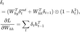
LaTeX: \delta_t=(W_{hy}^{T}\delta_t^{out}+W_{hh}^{T}\delta_{t+1})\odot(1-h_t^2),\quad \frac{\partial L}{\partial W_{hh}}=\sum_t\delta_t h_{t-1}^{T}

The tanh derivative is 1−h². Repeated multiplication by recurrent weights and activation derivatives may shrink gradients toward zero or amplify them greatly. Early words then receive a weak learning signal or updates become unstable. Gated architectures help long-context learning; suitable initialization and learning rates help training; clipping limits exploding gradients. Truncated BPTT restricts the backward time window to reduce computation and memory. It does not mean creating independent weights for each time step.

Diagram: BPTT follows this unrolled network backwards and sums gradients of shared weights. Labels: RNN | Output p1 | Input x1 | t = 1 | h1 | RNN | Output p2 | Input x2 | t = 2 | h2 | RNN | Output p3 | Input x3 | t = 3 | h0 | Shared weights at all steps; forward → and backward through time ←

Replace the vanilla cell with an LSTM or GRU while preserving a suitable sequence output. An LSTM introduces cell state and learned forget, input, output gates; a GRU introduces reset/update gates and a gated hidden-state mixture. These paths make retaining long context easier. Tune initialization and learning rate and inspect gradients.

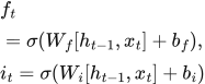
An LSTM contains a cell state C and hidden state h. Sigmoid gates control the fractions of information retained, admitted and exposed; a tanh transform proposes new content.

LaTeX: f_t=\sigma(W_f[h_{t-1},x_t]+b_f),\quad i_t=\sigma(W_i[h_{t-1},x_t]+b_i)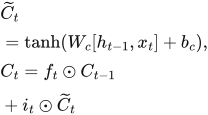

LaTeX: \widetilde C_t=\tanh(W_c[h_{t-1},x_t]+b_c),\quad C_t=f_t\odot C_{t-1}+i_t\odot\widetilde C_t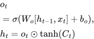

LaTeX: o_t=\sigma(W_o[h_{t-1},x_t]+b_o),\quad h_t=o_t\odot\tanh(C_t)

Diagram: The cell path retains selected old content and adds selected new content. Labels: C previous | × | + | C new | tanh | × | h | new | σ: f | σ: i | tanh: C~ | σ: o | × | [h previous, x current] | Each gate has its own learned weights and bias.

The forget gate f near 1 retains old content; near 0 removes it. The input gate i controls candidate admission. The output gate o selects the visible state. The additive cell path helps useful information and training signals travel over longer intervals, especially when forget gates retain relevant components.

In language modeling, the cell can retain an earlier subject while intervening words modify other features. When the topic changes, a learned forget gate can reduce obsolete information while the input gate admits new context. These are intuitive interpretations, not numeric gate values derivable from words alone. Exact values require weights, inputs and previous states. LSTMs often learn longer dependencies more effectively than vanilla RNNs, but do not guarantee perfect indefinite memory.