Deep Learning · TEE · section

R23 Q3b

Re examination January 2023 fully solved

Question

Question (10 marks). For input [0.5,0.7,0.8], first-stage multipliers [0.3,0.4,0.6], next receiving rows [0.5,0.2,0.3], [0.3,0.3,0.3], output rows [0.3,0.2], [0.2,0.3], use ReLU in the first two stages and sigmoid at outputs. Targets [0,1], zero biases, η = 0.1. Find predictions, MSE and all four hidden-to-output weight updates.

Answer — step by step

Given

For input [0.5,0.7,0.8], first-stage multipliers [0.3,0.4,0.6], next receiving rows [0.5,0.2,0.3], [0.3,0.3,0.3], output rows [0.3,0.2], [0.2,0.3], use ReLU in the first two stages and sigmoid at outputs.

Targets [0,1], zero biases, η = 0.1.

To find

Find all preactivations, hidden activations and final outputs. Calculate MSE and its output derivatives. Find the sigmoid output and, if requested, its derivative. Find the requested deltas and parameter gradients, then update the specified parameters.

Formula — which one and why

Forward propagation. Evaluate one layer completely before supplying its activated outputs to the next layer. Each layer has its own weights and biases.

x = input vector; h = hidden outputs; W₁,b₁ = hidden parameters; W₂,b₂ = output parameters; f₁,f₂ = the stated activations.

$z_h=W_1x+b_1$ LaTeX: z_h=W_1x+b_1

$h=f_1(z_h)$ LaTeX: h=f_1(z_h)

$z_o=W_2h+b_2$ LaTeX: z_o=W_2h+b_2

$o=f_2(z_o)$ LaTeX: o=f_2(z_o)

Yaad rakhne ka cue: Pehli layer ka activated output hi agli layer ka input hai.

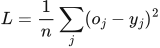
Mean squared loss. Average the squared scalar prediction errors. The derivative retains the factor 2/n; n must count the outputs included in this mean.

n = number of scalar prediction errors in the stated mean; oⱼ = prediction; yⱼ = target.

$L=\frac1n\sum_j(o_j-y_j)^2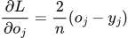$ LaTeX: L=\frac1n\sum_j(o_j-y_j)^2

$\frac{\partial L}{\partial o_j}=\frac2n(o_j-y_j)$ LaTeX: \frac{\partial L}{\partial o_j}=\frac2n(o_j-y_j)

Yaad rakhne ka cue: MSE mein derivative 2/n times error; half SSE ka rule blindly mat lagao.

Sigmoid and its slope. Use sigmoid when the neuron is specified to squash its preactivation into (0,1). Once its output is known, its derivative needs only output × (1−output).

z = preactivation; p = sigmoid output; e is the exponential base, not a prediction error in this formula.

$p=\frac{1}{1+e^{-z}}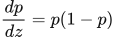$ LaTeX: p=\frac{1}{1+e^{-z}}

$\frac{dp}{dz}=p(1-p)$ LaTeX: \frac{dp}{dz}=p(1-p)

Yaad rakhne ka cue: Sigmoid output p; uska slope p × (1−p).

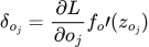
Backpropagation. The loss tells us how each output must change. Multiply by that neuron’s activation slope to obtain its delta. A weight gradient is receiving delta × sending value. Hidden deltas must include every outgoing path.

δ (delta) = derivative of loss with respect to a neuron’s preactivation; f′ = activation derivative; aᵢ = sending activation; Wⱼᵢ = connection weight. Use the exact loss scaling in the question.

$\delta_{o_j}=\frac{\partial L}{\partial o_j}f_o\prime(z_{o_j})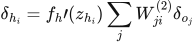$ LaTeX: \delta_{o_j}=\frac{\partial L}{\partial o_j}f_o\prime(z_{o_j})

$\delta_{h_i}=f_h\prime(z_{h_i})\sum_jW_{ji}^{(2)}\delta_{o_j}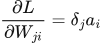$ LaTeX: \delta_{h_i}=f_h\prime(z_{h_i})\sum_jW_{ji}^{(2)}\delta_{o_j}

$\frac{\partial L}{\partial W_{ji}}=\delta_ja_i$ LaTeX: \frac{\partial L}{\partial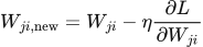 W_{ji}}=\delta_ja_i

$\frac{\partial L}{\partial b_j}=\delta_j$ LaTeX: \frac{\partial L}{\partial b_j}=\delta_j

$W_{ji,\mathrm{new}}=W_{ji}-\eta\frac{\partial L}{\partial W_{ji}}$ LaTeX: W_{ji,\mathrm{new}}=W_{ji}-\eta\frac{\partial L}{\partial W_{ji}}

Yaad rakhne ka cue: Receiving delta × sending value = us connection ka gradient.

Solution — step by step

Step 1: evaluate the first ReLU stage

The raw feature products are [0.5 × 0.3, 0.7 × 0.4, 0.8 × 0.6] = [0.15, 0.28, 0.48]. All are positive, so ReLU leaves them unchanged. Biases are zero.

Step 2: evaluate the second ReLU stage

h₁ = max(0, 0.5(0.15) + 0.2(0.28) + 0.3(0.48)) = max(0, 0.075 + 0.056 + 0.144) = 0.275.

h₂ = max(0, 0.3(0.15) + 0.3(0.28) + 0.3(0.48)) = max(0, 0.045 + 0.084 + 0.144) = 0.273.

Step 3: evaluate both sigmoid outputs

z₁ = 0.3(0.275) + 0.2(0.273) = 0.1371; o₁ = σ(z₁) = 0.534221413.

z₂ = 0.2(0.275) + 0.3(0.273) = 0.1369; o₂ = σ(z₂) = 0.534171647.

Step 4: calculate MSE and the output deltas

MSE = [(o₁ − 0)² + (o₂ − 1)²]/2 = 0.251194286. There are exactly two output components, so the square derivative's factor 2 cancels the division by 2.

δ₁ = (o₁ − 0)o₁(1 − o₁) = 0.132929724.

δ₂ = (o₂ − 1)o₂(1 − o₂) = −0.115913140.

Step 5: calculate each output-weight gradient

A weight gradient equals its receiving output delta multiplied by its sending hidden activation. Use the same old forward pass for all four connections.

Connection	Gradient calculation	Gradient
h₁ → o₁	0.132929724 × 0.275	0.036555674
h₂ → o₁	0.132929724 × 0.273	0.036289815
h₁ → o₂	−0.115913140 × 0.275	−0.031876113
h₂ → o₂	−0.115913140 × 0.273	−0.031644287

Step 6: subtract learning rate times each gradient

Connection	Update at η = 0.1	New weight
h₁ → o₁	0.3 − 0.1(0.036555674)	0.296344433
h₂ → o₁	0.2 − 0.1(0.036289815)	0.196371019
h₁ → o₂	0.2 − 0.1(−0.031876113)	0.203187611
h₂ → o₂	0.3 − 0.1(−0.031644287)	0.303164429

Final answer: predictions [0.534221413, 0.534171647], MSE 0.251194286, and output-weight rows [0.296344433, 0.196371019], [0.203187611, 0.303164429]. The positive gradients decrease weights feeding output 1, while the negative gradients increase weights feeding output 2.