Deep Learning · TEE · section
Rehearsal Q5b
Complete TEE paper rehearsal
Question (10 marks). Explain AdaGrad, give its update rule and discuss advantages and disadvantages compared with standard SGD.
Complete worked answer.
AdaGrad gives each parameter its own effective learning rate based on the sum of its past squared gradients. Start G₀ = 0, choose η and a small positive ε, then apply elementwise:
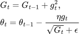 LaTeX:
G_t=G_{t-1}+g_t^2,\quad\theta_t=\theta_{t-1}-\frac{\eta g_t}{\sqrt{G_t}+\epsilon}Frequently updated coordinates accumulate a larger G and take smaller steps. Rarely active coordinates keep a relatively larger effective learning rate, which can be useful for sparse features. The square removes the sign in the accumulator; the unsquared current gradient still determines the direction of the parameter change.
Example with θ₀ = 1, η = 0.1, gradients 2 then 1 and negligible ε: first G = 4, denominator = 2, change = 0.1 × 2/2 = 0.1, θ₁ = 0.9. Next G = 5, denominator = √5 = 2.236068, change = 0.1/2.236068 = 0.04472136, θ₂ = 0.85527864.
Advantages over ordinary SGD include coordinatewise adaptation and usefulness for sparse gradients. Disadvantages include extra accumulator memory and continuously shrinking effective learning rates: G never decreases, so learning may become too slow. AdaGrad still requires a base learning rate and does not guarantee a global minimum. RMSProp addresses indefinite accumulation by replacing the sum with an exponentially weighted average.