Deep Learning · TEE · section
R25 Q2b · Vanishing/exploding gradients and GRU
February 2025 re-exam · complete solved paper
Question
Question. Explain vanishing/exploding gradients in RNNs and the gates of a GRU. (10 marks)
Answer — step by step
Definition. Vanishing and exploding gradients describe the attenuation or amplification of backward derivatives through repeated Jacobian products. In recurrent networks, these products extend across time and affect long-range credit assignment.
Explanation and working
In BPTT, the gradient repeatedly multiplies recurrent weights and activation derivatives. Products of many small factors can approach zero; early information then receives very little learning signal. Large repeated factors can make the gradient explode. These are about training signals, not an instruction that every hidden-state value must become zero or infinity.
Numerical intuition: 0.5¹⁰ = 0.0009765625, whereas 2¹⁰ = 1,024. Sigmoid's derivative is at most 0.25 and becomes even smaller in saturation. Tanh also saturates for large magnitude inputs.
Useful remedies include LSTM or GRU gates and cell paths, suitable initialization and learning rate, and gradient clipping for explosion. Clipping does not by itself solve vanishing gradients. LSTM makes long-range learning easier; it does not guarantee perfect unlimited memory.
Why the effect grows with sequence length
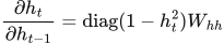
For a vanilla tanh RNN, each hidden-state transition contributes a Jacobian. The derivative through several transitions contains a product of these Jacobians:
 LaTeX:
\frac{\partial h_t}{\partial h_{t-1}}=\operatorname{diag}(1-h_t^2)W_{hh}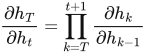 LaTeX:
\frac{\partial h_T}{\partial h_t}=\prod_{k=T}^{t+1}\frac{\partial h_k}{\partial h_{k-1}}The product is ordered from the latest transition toward the earliest. Small activation derivatives and recurrent transformations can attenuate the signal; repeated amplification can make it grow. A one-dimensional product illustrates the issue, but a vector RNN depends on the full matrix products, not one weight alone.
Gradient norm clipping: a complete numerical
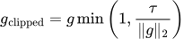
Norm clipping rescales an oversized gradient while retaining its direction. It limits the update size caused by an exploding gradient.
 LaTeX:
g_{\mathrm{clipped}}=g\min\left(1,\frac{\tau}{\lVert g\rVert_2}\right)If g is the zero vector, leave it unchanged. The threshold τ is positive. This is global norm clipping for the vector being considered; elementwise clipping is a different operation.
Question. A gradient is g = [6, 8]ᵀ. Clip its Euclidean norm to at most τ = 5, then update w = [1, 1]ᵀ with learning rate η = 0.1.
Given
Gradient g = [6,8]ᵀ; norm threshold τ = 5.
Old weights w = [1,1]ᵀ; η = 0.1.
To find
Find the clipped gradient and updated weights.
Formula — which one and why
Gradient norm clipping. If the vector norm exceeds the allowed threshold, multiply every component by the same scale. This changes magnitude while preserving direction.
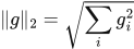
g = gradient vector; τ (tau) = maximum norm; ||g||₂ = square root of the sum of squared components; η = learning rate.
 LaTeX:
\lVert g\rVert_2=\sqrt{\sum_i g_i^2}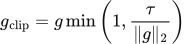 LaTeX:
g_{\mathrm{clip}}=g\min\left(1,\frac\tau{\lVert g\rVert_2}\right) LaTeX:
w_{\mathrm{new}}=w-\eta g_{\mathrm{clip}}Yaad rakhne ka cue: Bada gradient? Sab components ko ek hi factor se chhota karo.
Solution — step by step
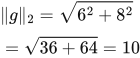
Step 1: calculate the original norm.
 LaTeX:
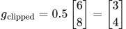
\lVert g\rVert_2=\sqrt{6^2+8^2}=\sqrt{36+64}=10Step 2: find the scale. Since 10 > 5, scale the vector by 5/10 = 0.5.
 LaTeX:
g_{\mathrm{clipped}}=0.5\begin{bmatrix}6\\8\end{bmatrix}=\begin{bmatrix}3\\4\end{bmatrix}Step 3: verify the clipped norm.
 LaTeX:
\sqrt{3^2+4^2}=\sqrt{9+16}=5Step 4: update each parameter with the clipped gradient.
 LaTeX:
w_{1,\mathrm{new}}=1-0.1(3)=0.7 LaTeX:
w_{2,\mathrm{new}}=1-0.1(4)=0.6Final answer: clipped gradient [3, 4]ᵀ and new weights [0.7, 0.6]ᵀ. Clipping does not increase a vanishing gradient and does not replace the need for an appropriate recurrent architecture.
Gradient norm clipping: [3, 4]
Question. Clip gradient g = [3, 4] to maximum L2 norm 10. Use global norm clipping.
Given
g = [3, 4]; threshold τ = 10.
To find
The norm, scaling factor and clipped gradient.
Formula — which one and why
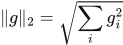
Global norm clipping scales the entire list by one common factor only if its norm exceeds the threshold.
τ is the maximum permitted norm, not a per-entry bound.
 LaTeX:
\|g\|_2=\sqrt{\sum_i g_i^2} LaTeX:
g_{\mathrm{clip}}=g\min(1,\tau/\|g\|_2)Yaad rakhne ka cue: Norm bada ho tab sab entries ko same ratio se chhota karo.
Solution — step by step
Step 1: calculate the squared norm.
 LaTeX:
3^2+4^2=25Step 2: take the square root.
 LaTeX:
\|g\|_2=\sqrt{25}=5Step 3: choose the shared scale.
 LaTeX:
c=\min(1,10/5)=1Step 4: scale every entry.
 LaTeX:
g_1^{\mathrm{clip}}=3(1)=3 LaTeX:
g_2^{\mathrm{clip}}=4(1)=4Final answer: Clipped gradient = [3, 4].
Gradient norm clipping: [0, 12]
Question. Clip gradient g = [0, 12] to maximum L2 norm 3. Use global norm clipping.
Given
g = [0, 12]; threshold τ = 3.
To find
The norm, scaling factor and clipped gradient.
Formula — which one and why
Global norm clipping scales the entire list by one common factor only if its norm exceeds the threshold.
τ is the maximum permitted norm, not a per-entry bound.
LaTeX: \|g\|_2=\sqrt{\sum_i g_i^2}LaTeX: g_{\mathrm{clip}}=g\min(1,\tau/\|g\|_2)Yaad rakhne ka cue: Norm bada ho tab sab entries ko same ratio se chhota karo.
Solution — step by step
Step 1: calculate the squared norm.
 LaTeX:
0^2+12^2=144Step 2: take the square root.
 LaTeX:
\|g\|_2=\sqrt{144}=12Step 3: choose the shared scale.
 LaTeX:
c=\min(1,3/12)=0.25Step 4: scale every entry.
 LaTeX:
g_1^{\mathrm{clip}}=0(0.25)=0 LaTeX:
g_2^{\mathrm{clip}}=12(0.25)=3Final answer: Clipped gradient = [0.0, 3.0].
Definition. A gated recurrent unit (GRU) is a recurrent architecture that uses reset and update gates to control its hidden-state transition. Unlike a standard LSTM, it does not carry a separate cell state alongside the hidden state.
Gate equations and the convention used here
The reset gate r controls how the previous hidden state enters candidate formation. The update gate z controls the mixture of the old state and the candidate. Both are calculated from the current input and previous hidden state:
 LaTeX:
r_t=\sigma(W_rx_t+U_rh_{t-1}+b_r) LaTeX:
z_t=\sigma(W_zx_t+U_zh_{t-1}+b_z)The candidate equation used in these notes applies reset before the recurrent candidate transformation:
 LaTeX:
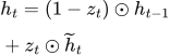
\widetilde h_t=\tanh(W_hx_t+U_h(r_t\odot h_{t-1})+b_h)These notes define z as the fraction of new candidate admitted:
 LaTeX:
h_t=(1-z_t)\odot h_{t-1}+z_t\odot\widetilde h_tThus z near 0 favors retention of the old hidden state, while z near 1 favors the candidate. The reset gate affects the candidate calculation; it does not directly multiply the retained old-state term in the final mixture.
Complete numerical with supplied gate values
Question. A scalar GRU has hₜ₋₁ = 0.4, reset gate rₜ = 0.5, update gate zₜ = 0.25, xₜ = 1, Wₕ = 0.2, Uₕ = 0.5 and bₕ = 0. Calculate the candidate and new hidden state using hₜ = (1−zₜ)hₜ₋₁ + zₜh̃ₜ.
Given
Old hidden state = 0.4; r = 0.5; z = 0.25.
x = 1; W = 0.2; U = 0.5; b = 0.
Here z weights the candidate in the final mixture.
To find
Find candidate and new hidden state.
Formula — which one and why
GRU reset and state mixture. The reset gate controls old-state information entering the candidate. The stated update convention then mixes the original old state and the candidate.
r = reset gate; z = update gate; h_old = previous state; h_tilde = candidate. Here z weights the candidate; some questions instead define z to weight the old state.
 LaTeX:
\widetilde h=\tanh(Wx+U(r\odot h_{\mathrm{old}})+b) LaTeX:
h=(1-z)\odot h_{\mathrm{old}}+z\odot\widetilde hYaad rakhne ka cue: Reset candidate ko control; update gate old-new mixture ko control.
Solution — step by step
Step 1: apply the reset gate to the previous hidden state.
 LaTeX:
r_th_{t-1}=0.5(0.4)=0.2The gates are already supplied as outputs, so no further sigmoid calculation is needed.
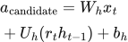
Step 2: calculate the candidate preactivation.
 LaTeX:
a_{\mathrm{candidate}}=W_hx_t+U_h(r_th_{t-1})+b_h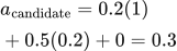 LaTeX:
a_{\mathrm{candidate}}=0.2(1)+0.5(0.2)+0=0.3Step 3: apply tanh to obtain the candidate.
 LaTeX:
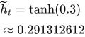
\widetilde h_t=\tanh(0.3)\approx0.291312612Step 4: calculate the two mixture contributions.
 LaTeX:
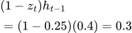
(1-z_t)h_{t-1}=(1-0.25)(0.4)=0.3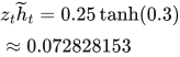 LaTeX:
z_t\widetilde h_t=0.25\tanh(0.3)\approx0.072828153Step 5: add the contributions.
 LaTeX:
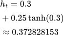
h_t=0.3+0.25\tanh(0.3)\approx0.372828153Final answer: candidate ≈ 0.291313 and new hidden state ≈ 0.372828. The new scalar state lies between the old state 0.4 and the candidate 0.291313, as expected for this convex mixture.
If the question uses the other update-gate convention
Some texts define z as the fraction of the old state retained:
 LaTeX:
h_t=z_th_{t-1}+(1-z_t)\widetilde h_tUnder that explicitly different convention, the same numerical value z = 0.25 gives:
 LaTeX:
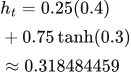
h_t=0.25(0.4)+0.75\tanh(0.3)\approx0.318484459This is not the answer to the worked question above, which states the first convention. To represent an identical mixture while switching conventions, the gate values must be complemented as well. Always identify the final mixture equation before substituting values.
Relationship to LSTM
A basic GRU has three affine transformations: reset, update and candidate. A standard LSTM has four: forget, input, output and candidate. With equal input and hidden dimensions and the same bias convention, GRU therefore has fewer recurrent parameters. This is a parameter-count comparison, not a guarantee of higher accuracy or faster execution for every task.
Retain-old GRU with gate 0
Question. Use h_new = z h_old+(1−z) candidate. Given h_old = 0.4, z = 0, r = 0.5, x = 1, W = 0.2, U = 0.5 and b = 0, calculate the candidate and new state.
Given
h_old = 0.4; z = 0; r = 0.5; x = 1.
W = 0.2; U = 0.5; b = 0; z is the retain-old gate.
To find
Candidate and final hidden state.
Formula — which one and why
The reset gate changes old-state input to the candidate. The update gate separately mixes the original old state and candidate.
The question explicitly makes z multiply the old state. r and z do different jobs.
 LaTeX:
\widetilde h=\tanh(Wx+U(rh_{\mathrm{old}})+b) LaTeX:
h_{\mathrm{new}}=zh_{\mathrm{old}}+(1-z)\widetilde hYaad rakhne ka cue: Reset sirf candidate mein; update mix mein original old state.
Solution — step by step
Step 1: reset the old state for candidate formation.
 LaTeX:
rh_{\mathrm{old}}=0.5(0.4)=0.2Step 2: calculate the candidate raw sum.
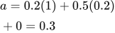 LaTeX:
a=0.2(1)+0.5(0.2)+0=0.3Step 3: apply tanh.
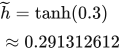 LaTeX:
\widetilde h=\tanh(0.3)\approx0.291312612Step 4: retain the old-state fraction.
 LaTeX:
0(0.4)=0Step 5: calculate the candidate fraction.
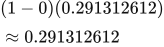 LaTeX:
(1-0)(0.291312612)\approx0.291312612Step 6: add the two fractions.
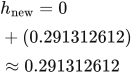 LaTeX:
h_{\mathrm{new}}=0+(0.291312612)\approx0.291312612Final answer: Candidate ≈ 0.291312612; new state ≈ 0.291312612.
Retain-old GRU with gate 0.8
Question. Use h_new = z h_old+(1−z) candidate. Given h_old = -0.2, z = 0.8, r = 0.5, x = 1, W = 0.2, U = 0.5 and b = 0, calculate the candidate and new state.
Given
h_old = -0.2; z = 0.8; r = 0.5; x = 1.
W = 0.2; U = 0.5; b = 0; z is the retain-old gate.
To find
Candidate and final hidden state.
Formula — which one and why
The reset gate changes old-state input to the candidate. The update gate separately mixes the original old state and candidate.
The question explicitly makes z multiply the old state. r and z do different jobs.
LaTeX: \widetilde h=\tanh(Wx+U(rh_{\mathrm{old}})+b)LaTeX: h_{\mathrm{new}}=zh_{\mathrm{old}}+(1-z)\widetilde hYaad rakhne ka cue: Reset sirf candidate mein; update mix mein original old state.
Solution — step by step
Step 1: reset the old state for candidate formation.
 LaTeX:
rh_{\mathrm{old}}=0.5(-0.2)=-0.1Step 2: calculate the candidate raw sum.
 LaTeX:
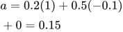
a=0.2(1)+0.5(-0.1)+0=0.15Step 3: apply tanh.
 LaTeX:
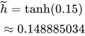
\widetilde h=\tanh(0.15)\approx0.148885034Step 4: retain the old-state fraction.
 LaTeX:
0.8(-0.2)=-0.16Step 5: calculate the candidate fraction.
 LaTeX:
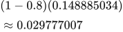
(1-0.8)(0.148885034)\approx0.029777007Step 6: add the two fractions.
 LaTeX:
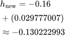
h_{\mathrm{new}}=-0.16+(0.029777007)\approx-0.130222993Final answer: Candidate ≈ 0.148885034; new state ≈ -0.130222993.