Deep Learning · TEE · section
Backpropagation with one hidden neuron
Neural-network foundations
Definition. Backpropagation computes the derivatives of a scalar objective with respect to network parameters by applying the chain rule in reverse through the computational graph. An optimizer then uses these derivatives to update the parameters.
Network equations and the meaning of delta
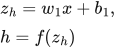
Consider one input, one hidden neuron and one output neuron:
 LaTeX:
z_h=w_1x+b_1,\qquad h=f(z_h)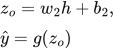 LaTeX:
z_o=w_2h+b_2,\qquad\hat y=g(z_o)For the half squared loss used in this example:
 LaTeX:
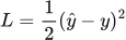
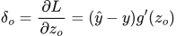
L=\frac12(\hat y-y)^2Define a neuron's delta as the derivative of the loss with respect to its preactivation, not with respect to its output:
 LaTeX:
\delta_o=\frac{\partial L}{\partial z_o}=(\hat y-y)g'(z_o)The output-weight derivative contains the hidden activation because zₒ = w₂h + b₂:
 LaTeX:
\frac{\partial L}{\partial w_2}=\delta_o h,\qquad\frac{\partial L}{\partial b_2}=\delta_oTo reach the hidden neuron, continue backwards through the old output weight and the hidden activation:
 LaTeX:
\delta_h=\delta_o w_2 f'(z_h) LaTeX:
\frac{\partial L}{\partial w_1}=\delta_h x,\qquad\frac{\partial L}{\partial b_1}=\delta_hThe bias derivative equals the corresponding delta because the derivative of z with respect to its additive bias is 1. All these derivatives belong to the same forward pass; an updated weight must not be used partway through this backward pass.
Complete worked numerical
Question. x = 2, y = 1; w₁ = 0.5, b₁ = 0.1; w₂ = 0.8, b₂ = 0.2. Both neurons use ReLU. Use half squared loss. Find the output and all four parameter gradients, then update all four parameters using η = 0.1.
Given
x = 2, y = 1.
w₁ = 0.5, b₁ = 0.1.
w₂ = 0.8, b₂ = 0.2.
Both neurons use ReLU.
Use half squared loss.
Find the output and all four parameter gradients, then update all four parameters using η = 0.1.
To find
Find all preactivations, hidden activations and final outputs. Calculate the half summed squared loss and its output derivatives. Find the requested deltas and parameter gradients, then update the specified parameters.
Formula — which one and why
Forward propagation. Evaluate one layer completely before supplying its activated outputs to the next layer. Each layer has its own weights and biases.
x = input vector; h = hidden outputs; W₁,b₁ = hidden parameters; W₂,b₂ = output parameters; f₁,f₂ = the stated activations.
 LaTeX:
z_h=W_1x+b_1 LaTeX:
h=f_1(z_h) LaTeX:
z_o=W_2h+b_2 LaTeX:
o=f_2(z_o)Yaad rakhne ka cue: Pehli layer ka activated output hi agli layer ka input hai.
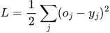
Half summed squared loss. This loss convention takes one-half of the sum of squared prediction errors. Use it when the question specifies it, or explicitly state it as an assumption when the paper omits the loss. Differentiating cancels the factor one-half against the square derivative.
oⱼ = output j; yⱼ = target j; L = half summed squared loss under the stated or explicitly assumed convention.
 LaTeX:
L=\frac12\sum_j(o_j-y_j)^2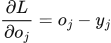 LaTeX:
\frac{\partial L}{\partial o_j}=o_j-y_jYaad rakhne ka cue: Half aur square ka 2 cancel: output derivative = prediction − target.
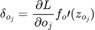
Backpropagation. The loss tells us how each output must change. Multiply by that neuron’s activation slope to obtain its delta. A weight gradient is receiving delta × sending value. Hidden deltas must include every outgoing path.
δ (delta) = derivative of loss with respect to a neuron’s preactivation; f′ = activation derivative; aᵢ = sending activation; Wⱼᵢ = connection weight. Use the exact loss scaling in the question.
 LaTeX:
\delta_{o_j}=\frac{\partial L}{\partial o_j}f_o\prime(z_{o_j})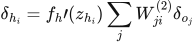 LaTeX:
\delta_{h_i}=f_h\prime(z_{h_i})\sum_jW_{ji}^{(2)}\delta_{o_j}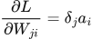 LaTeX:
\frac{\partial L}{\partial W_{ji}}=\delta_ja_i LaTeX:
\frac{\partial L}{\partial b_j}=\delta_j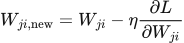 LaTeX:
W_{ji,\mathrm{new}}=W_{ji}-\eta\frac{\partial L}{\partial W_{ji}}Yaad rakhne ka cue: Receiving delta × sending value = us connection ka gradient.
Solution — step by step
Step 1: forward propagation through the hidden neuron.
 LaTeX:
z_h=0.5(2)+0.1=1.1 LaTeX:
h=\operatorname{ReLU}(1.1)=1.1Step 2: forward propagation through the output neuron.
 LaTeX:
z_o=0.8(1.1)+0.2=1.08 LaTeX:
\hat y=\operatorname{ReLU}(1.08)=1.08ReLU is not bounded above by 1, so this output is valid. It is not being interpreted as a probability here.
Step 3: calculate the loss and output delta.
 LaTeX:
L=\frac12(1.08-1)^2=0.0032Both preactivations are positive, so both ReLU derivatives are 1.
 LaTeX:
\delta_o=(1.08-1)(1)=0.08Step 4: calculate the output-layer parameter gradients.
 LaTeX:
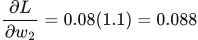
\frac{\partial L}{\partial w_2}=0.08(1.1)=0.088 LaTeX:
\frac{\partial L}{\partial b_2}=0.08Step 5: propagate the derivative to the hidden neuron.
Use w₂ = 0.8, its value during the forward pass:
 LaTeX:
\delta_h=0.08(0.8)(1)=0.064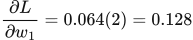 LaTeX:
\frac{\partial L}{\partial w_1}=0.064(2)=0.128 LaTeX:
\frac{\partial L}{\partial b_1}=0.064Step 6: update each parameter using its own gradient.
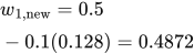 LaTeX:
w_{1,\mathrm{new}}=0.5-0.1(0.128)=0.4872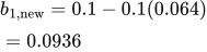 LaTeX:
b_{1,\mathrm{new}}=0.1-0.1(0.064)=0.0936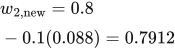 LaTeX:
w_{2,\mathrm{new}}=0.8-0.1(0.088)=0.7912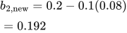 LaTeX:
b_{2,\mathrm{new}}=0.2-0.1(0.08)=0.192| Parameter | Gradient from the original forward pass | Updated value |
|---|---|---|
| w₁ | 0.128 | 0.4872 |
| b₁ | 0.064 | 0.0936 |
| w₂ | 0.088 | 0.7912 |
| b₂ | 0.08 | 0.192 |
Final answer: the original prediction is 1.08 and its loss is 0.0032. The table contains all requested gradients and updated parameters. A new forward pass would use all four new parameters together.