Deep Learning · TEE · section
Adam remembers both direction and squared size
Optimization algorithms
Definition. Adam, or adaptive moment estimation, uses bias-corrected exponentially weighted estimates of the first moment and the uncentered second moment of gradients to calculate parameter-specific updates.
What the two states represent
| State or coefficient | Meaning |
|---|---|
| mₜ | Moving average of signed gradients; retains directional information |
| sₜ | Moving average of squared gradients; estimates their uncentered second moment |
| β₁ | Decay coefficient for the first-moment estimate |
| β₂ | Decay coefficient for the second-moment estimate |
| t | Update number, starting at 1 for the first update |
| η and ε | Base learning rate and small denominator stabilizer |
The second moment is not the variance: it averages g² without subtracting a mean. Both states start at zero unless specified otherwise. These notes use s throughout this lesson; texts that use v for Adam's second moment mean the same state, not momentum's displacement velocity.
Recurrences, bias correction and update
 LaTeX:
m_t=\beta_1m_{t-1}+(1-\beta_1)g_t LaTeX:
s_t=\beta_2s_{t-1}+(1-\beta_2)g_t^2Zero initialization reduces the total weight initially attached to observed gradients. Divide by the appropriate accumulated observation weight:
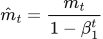 LaTeX:
\hat m_t=\frac{m_t}{1-\beta_1^t} LaTeX:
\hat s_t=\frac{s_t}{1-\beta_2^t}The update uses the corrected signed average in the numerator and the root of the corrected squared-gradient average in the denominator:
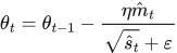 LaTeX:
\theta_t=\theta_{t-1}-\frac{\eta\hat m_t}{\sqrt{\hat s_t}+\varepsilon}The derivation in the next lesson explains why the correction factors contain powers of the iteration number. No additional multiplication by gₜ belongs in this final update: its contribution is already inside mₜ.
Complete numerical: changing gradient magnitude
Question. θ₀ = 1, m₀ = s₀ = 0, η = 0.1, β₁ = 0.9, β₂ = 0.999. Given g₁ = 2 and g₂ = 1, find two Adam updates, neglecting epsilon only in the numerical arithmetic.
Given
θ₀ = 1; initial state(s) = 0; η = 0.1.
Supplied gradients g₁ = 2, g₂ = 1.
ε = 0 for this hand calculation.
β₁ = 0.9; β₂ = 0.999; use bias correction.
To find
Calculate all required states and the parameter after each of two updates.
Formula — which one and why
Adam with bias correction. Keep two states: one averages signed gradients, the other averages squared gradients. Correct their initial bias toward zero before combining them in the parameter update.
m = signed average; s (also written v) = squared average; β₁ and β₂ = retained fractions; t = iteration number. A hat marks a corrected value. Carry raw m and s into the next recurrence.
LaTeX: m_t=\beta_1m_{t-1}+(1-\beta_1)g_tLaTeX: s_t=\beta_2s_{t-1}+(1-\beta_2)g_t^2LaTeX: \hat m_t=\frac{m_t}{1-\beta_1^t}LaTeX: \hat s_t=\frac{s_t}{1-\beta_2^t}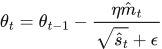 LaTeX:
\theta_t=\theta_{t-1}-\frac{\eta\hat m_t}{\sqrt{\hat s_t}+\epsilon}Yaad rakhne ka cue: Direction memory + square memory; hats lagao, phir update.
Solution — step by step
Iteration 1 — step 1: update the two raw states.
 LaTeX:
m_1=0.9(0)+0.1(2)=0.2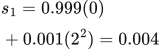 LaTeX:
s_1=0.999(0)+0.001(2^2)=0.004Step 2: correct both states using t = 1.
 LaTeX:
\hat m_1=\frac{0.2}{1-0.9^1}=\frac{0.2}{0.1}=2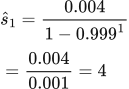 LaTeX:
\hat s_1=\frac{0.004}{1-0.999^1}=\frac{0.004}{0.001}=4Step 3: update the parameter.
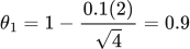 LaTeX:
\theta_1=1-\frac{0.1(2)}{\sqrt4}=0.9Start with the current gradient and the two states saved from the previous iteration.
Carry forward raw states: m = 0.2, s = 0.004. The corrected values are used for this update.
Iteration 2 — step 1: carry forward the raw states m₁ and s₁.
The recurrence uses the raw states 0.2 and 0.004, not the corrected values 2 and 4.
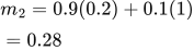 LaTeX:
m_2=0.9(0.2)+0.1(1)=0.28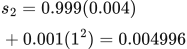 LaTeX:
s_2=0.999(0.004)+0.001(1^2)=0.004996Step 2: correct both states using t = 2.
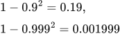 LaTeX:
1-0.9^2=0.19,\qquad1-0.999^2=0.001999 LaTeX:
\hat m_2=\frac{0.28}{0.19}\approx1.473684211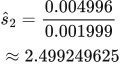 LaTeX:
\hat s_2=\frac{0.004996}{0.001999}\approx2.499249625Step 3: divide the corrected first moment by the corrected root.
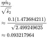 LaTeX:
\frac{\eta\hat m_2}{\sqrt{\hat s_2}}\approx\frac{0.1(1.473684211)}{\sqrt{2.499249625}}\approx0.093217964Step 4: update from θ₁.
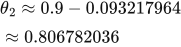 LaTeX:
\theta_2\approx0.9-0.093217964\approx0.806782036Start with the current gradient and the two states saved from the previous iteration.
Carry forward raw states: m = 0.28, s = 0.004996. The corrected values are used for this update.
| State | After iteration 1 | After iteration 2 |
|---|---|---|
| Raw first moment m | 0.2 | 0.28 |
| Raw second moment s | 0.004 | 0.004996 |
| Corrected first moment | 2 | 1.473684211 |
| Corrected second moment | 4 | 2.499249625 |
| Parameter θ | 0.9 | 0.806782036 |
Final answer: θ₁ = 0.9 and θ₂ ≈ 0.806782. Store the raw moments for the next recurrence and use the corrected moments for the current parameter update.
Properties and limitations
Adam combines directional averaging with coordinate-specific scaling, which can be useful with noisy or differently scaled gradients. It requires two state values per parameter in addition to the parameter itself. η, β₁, β₂ and ε remain hyperparameters. Faster reduction of training loss does not establish better generalization, and Adam does not guarantee the global optimum of a general neural-network objective.