Deep Learning · TEE · section

Momentum remembers movement

Optimization algorithms

Definition. Momentum is a gradient-based optimization method that combines the current gradient correction with a fraction of the previous parameter displacement. It can accumulate movement along persistent directions and damp some oscillations across alternating directions.

Update equations and convention

This course uses signed displacement velocity v. It already includes the learning rate, and the parameter update adds it to the old parameter:

$g_t=J'(\theta_{t-1})$ LaTeX: g_t=J'(\theta_{t-1})

$v_t=\beta v_{t-1}-\eta g_t$ LaTeX: v_t=\beta v_{t-1}-\eta g_t

$\theta_t=\theta_{t-1}+v_t$ LaTeX: \theta_t=\theta_{t-1}+v_t

θ is the parameter, η is the learning rate and β controls how much previous displacement is retained, normally with 0 ≤ β < 1. A negative v moves θ in the negative direction. Every parameter has its own velocity; this optimizer state is distinct from the network's trainable parameters.

Combine the retained displacement with the current gradient correction, then apply the resulting velocity to the old parameter. Tap the diagram to enlarge.

Complete numerical: two iterations

Question. J(θ) = ½θ², θ₀ = 1, v₀ = 0, η = 0.1, β = 0.9. Find two iterations using signed displacement velocity.

Given

J(θ) = ½θ²; θ₀ = 1; v₀ = 0.

η = 0.1; β = 0.9; signed-displacement velocity.

To find

Find the gradient, velocity and actual parameter after each of two iterations.

Formula — which one and why

Momentum with signed velocity. Combine the retained old displacement with the current downhill correction, then add that signed displacement to the old parameter.

v = signed velocity/displacement; β = momentum coefficient; g = current gradient; η = learning rate. This convention uses +v in the parameter update.

$v_t=\beta v_{t-1}-\eta g_t$ LaTeX: v_t=\beta v_{t-1}-\eta g_t

$\theta_t=\theta_{t-1}+v_t$ LaTeX: \theta_t=\theta_{t-1}+v_t

Yaad rakhne ka cue: Pehle velocity banao; phir old parameter mein velocity jodo.

Solution — step by step

Derivative used: differentiating J gives J′(θ) = θ. The gradient must therefore be reevaluated at the current θ on each iteration.

Step 1: Iteration 1: gradient, velocity, parameter.

$g_1=J'(1)=1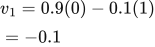$ LaTeX: g_1=J'(1)=1

$\theta_1=1+(-0.1)=0.9$ LaTeX: \theta_1=1+(-0.1)=0.9

Step 2: Iteration 2: use θ₁ and v₁.

$g_2=J'(0.9)=0.9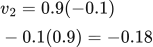$ LaTeX: g_2=J'(0.9)=0.9

$\theta_2=0.9+(-0.18)=0.72$ LaTeX: \theta_2=0.9+(-0.18)=0.72

Iteration	Parameter where gradient is evaluated	Gradient	New velocity	New parameter
1	1	1	−0.1	0.9
2	0.9	0.9	−0.18	0.72

Final answer: θ₁ = 0.9 and θ₂ = 0.72. At iteration 2, the retained displacement contributes −0.09 and the new gradient correction contributes another −0.09. Their sum explains the larger displacement despite the smaller current gradient.

Properties and alternative notation

Momentum can improve progress through long, poorly scaled valleys, but excessive learning rate or momentum can overshoot. It does not guarantee a global minimum for a general neural-network objective.

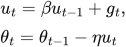
Some texts store a positive gradient accumulator u instead:

With constant η and consistent initialization, this corresponds to vₜ = −ηuₜ. A normalized moving average containing (1−β)gₜ is a different scaling convention. Use the exact recurrence stated in the question instead of combining pieces of different conventions.