Deep Learning · TEE · section
BPTT with every arithmetic step visible
Recurrent neural networks
Question. A scalar RNN uses the linear state equation hₜ = u xₜ + v hₜ₋₁ + b. Its prediction is ŷ = h₂ and its loss is L = ½(ŷ−1)². Given u = 0.2, v = 0.5, b = 0, h₀ = 0, x₁ = 1 and x₂ = 2, calculate the gradients of u, v and b using BPTT, then update them once using learning rate η = 0.1.
Given
hₜ = uxₜ+vhₜ₋₁+b; prediction = h₂.
u = 0.2; v = 0.5; b = 0; h₀ = 0; x₁ = 1; x₂ = 2.
Target = 1; half squared loss; η = 0.1.
To find
Find gradients for u,v,b and update each once.
Formula — which one and why
Backpropagation through time. Unroll the recurrence, send the loss derivative backward through its links and add contributions for each shared parameter before updating it once.
For h_t=ux_t+vh_(t−1)+b with loss only at the last state: δ_t = loss derivative at that state. The linear recurrence has activation slope 1.
 LaTeX:
\delta_T=h_T-y LaTeX:
\delta_t=v\delta_{t+1}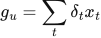 LaTeX:
g_u=\sum_t\delta_tx_t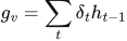 LaTeX:
g_v=\sum_t\delta_th_{t-1} LaTeX:
g_b=\sum_t\delta_tYaad rakhne ka cue: Time ke har use ka gradient jodo; shared weight ko ek baar update karo.
Gradient descent. Evaluate the gradient at the current parameter, multiply by the learning rate and subtract. If the objective is supplied, differentiate it and recompute the gradient after each update.
θ (theta) = trainable parameter; g = derivative of the stated objective J; η = learning rate; t labels the update number.
 LaTeX:
g_t=J\prime(\theta_{t-1}) LaTeX:
\theta_t=\theta_{t-1}-\eta g_tYaad rakhne ka cue: Naya = purana − learning rate × current gradient.
Solution — step by step
Model and dependency structure
u is the input weight, v is the recurrent weight and b is the hidden bias. Each is shared by both time steps. The hidden activation is linear in this question, so its derivative is 1. There is a loss only at time step 2; time step 1 influences that loss through h₂.
Step 1: complete the forward pass
 LaTeX:
h_1=ux_1+vh_0+b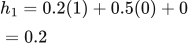 LaTeX:
h_1=0.2(1)+0.5(0)+0=0.2 LaTeX:
h_2=ux_2+vh_1+b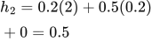 LaTeX:
h_2=0.2(2)+0.5(0.2)+0=0.5 LaTeX:
L=\frac12(0.5-1)^2=0.125Step 2: differentiate the loss at the final step
Because the output is h₂ and the state activation is linear:
 LaTeX:
\delta_2=\frac{\partial L}{\partial h_2}=h_2-1=-0.5Step 3: propagate the derivative to the earlier state
The local derivative of h₂ with respect to h₁ is the recurrent weight v = 0.5. Applying the chain rule:
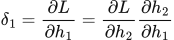 LaTeX:
\delta_1=\frac{\partial L}{\partial h_1}=\frac{\partial L}{\partial h_2}\frac{\partial h_2}{\partial h_1}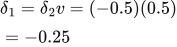 LaTeX:
\delta_1=\delta_2v=(-0.5)(0.5)=-0.25There is no separate direct loss at time step 1 to add here. Both deltas use the original recurrent weight.
Step 4: sum the contributions to each shared parameter
u appears in both h₁ and h₂, so its gradient receives one contribution from each use:
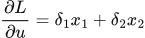 LaTeX:
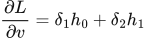
\frac{\partial L}{\partial u}=\delta_1x_1+\delta_2x_2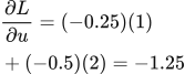 LaTeX:
\frac{\partial L}{\partial u}=(-0.25)(1)+(-0.5)(2)=-1.25For v, the sending activation is the previous hidden state at the corresponding time:
 LaTeX:
\frac{\partial L}{\partial v}=\delta_1h_0+\delta_2h_1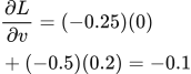 LaTeX:
\frac{\partial L}{\partial v}=(-0.25)(0)+(-0.5)(0.2)=-0.1The same additive bias is used at both steps. Its two local derivatives are 1:
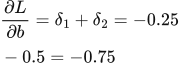 LaTeX:
\frac{\partial L}{\partial b}=\delta_1+\delta_2=-0.25-0.5=-0.75| Shared parameter | Contribution at time 1 | Contribution at time 2 | Total gradient |
|---|---|---|---|
| u | −0.25 × 1 = −0.25 | −0.5 × 2 = −1 | −1.25 |
| v | −0.25 × 0 = 0 | −0.5 × 0.2 = −0.1 | −0.1 |
| b | −0.25 | −0.5 | −0.75 |
Step 5: update each shared parameter once
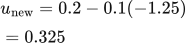 LaTeX:
u_{\mathrm{new}}=0.2-0.1(-1.25)=0.325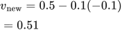 LaTeX:
v_{\mathrm{new}}=0.5-0.1(-0.1)=0.51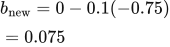 LaTeX:
b_{\mathrm{new}}=0-0.1(-0.75)=0.075Final answer: gradients are −1.25, −0.1 and −0.75; updated parameters are u = 0.325, v = 0.51 and b = 0.075.
Evaluate the updated model
Restart from the same h₀ = 0 and use all updated parameters together:
 LaTeX:
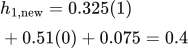
h_{1,\mathrm{new}}=0.325(1)+0.51(0)+0.075=0.4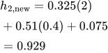 LaTeX:
h_{2,\mathrm{new}}=0.325(2)+0.51(0.4)+0.075=0.929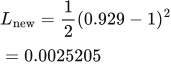 LaTeX:
L_{\mathrm{new}}=\frac12(0.929-1)^2=0.0025205The loss decreases in this particular update. That is consistent with the computed gradient, but a decrease is not guaranteed for every choice of learning rate.
Extension to a tanh RNN
For tanh, the derivative at each state transition also contains 1−hₜ². A trainable output layer contributes its own local derivatives. If losses occur at several time steps, add the direct output-loss contribution and the future-state contribution before applying the local activation derivative. Truncated BPTT limits the number of time steps traversed backward; it does not create separate copies of the recurrent parameters.
Second worked example: nonlinear tanh BPTT
Question. A scalar RNN uses hₜ = tanh(uxₜ + vhₜ₋₁ + b). Given u = 0.4, v = 0.3, b = 0.1, h₀ = 0 and inputs x₁ = 1, x₂ = −1, its final output is h₂ and target is 0.2. Use only the final-time loss L = ½(h₂ − 0.2)². Calculate both states, all three shared-parameter gradients and one simultaneous update at η = 0.1.
Given
Shared input weight u = 0.4; shared recurrent weight v = 0.3; shared bias b = 0.1. Initial state h₀ = 0; x₁ = 1, x₂ = −1. Hidden activation = tanh; final target = 0.2; learning rate η = 0.1. There is no separate output layer and no loss at time 1.
To find
Forward states h₁ and h₂, final loss, gradients with respect to u, v and b, and all three updated parameters.
Formula — which one and why
Backpropagation must pass through each tanh derivative. Because u, v and b are shared, add their local contributions from both time steps before updating them.
 LaTeX:
z_t=ux_t+vh_{t-1}+b,\qquad h_t=\tanh(z_t) LaTeX:
\delta_2=(h_2-y)(1-h_2^2),\qquad \delta_1=v\delta_2(1-h_1^2)LaTeX: \frac{\partial L}{\partial u}=\delta_1x_1+\delta_2x_2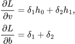 LaTeX:
\frac{\partial L}{\partial v}=\delta_1h_0+\delta_2h_1,\qquad \frac{\partial L}{\partial b}=\delta_1+\delta_2Here δₜ means ∂L/∂zₜ, not ∂L/∂hₜ. The factor v in δ₁ is the old recurrent weight 0.3. The derivative of tanh is 1 − hₜ², using that step's activated state.
Solution — step by step
Step 1: calculate the first state
z₁ = 0.4(1) + 0.3(0) + 0.1 = 0.5.
h₁ = tanh(0.5) = 0.462117157.
Step 2: carry that state into time 2
z₂ = 0.4(−1) + 0.3(0.462117157) + 0.1 = −0.161364853.
h₂ = tanh(−0.161364853) = −0.159978716.
Step 3: calculate the final loss and final-time delta
Prediction error h₂ − y = −0.159978716 − 0.2 = −0.359978716.
L = ½(−0.359978716)² = 0.064792338.
δ₂ = (−0.359978716)[1 − (−0.159978716)²] = −0.350765712.
Step 4: backpropagate through the recurrent connection and first tanh
There is no direct loss at time 1. Its gradient arrives entirely through time 2:
δ₁ = 0.3(−0.350765712)[1 − (0.462117157)²] = −0.082757670.
Step 5: sum each shared parameter's contributions over time
| Parameter | Time contributions | Total gradient |
|---|---|---|
| u | (−0.082757670)(1) + (−0.350765712)(−1) | 0.268008043 |
| v | (−0.082757670)(0) + (−0.350765712)(0.462117157) | −0.162094854 |
| b | −0.082757670 + (−0.350765712) | −0.433523382 |
For v, the sending state is hₜ₋₁: h₀ for time 1, h₁ for time 2. The negative second input makes its contribution to the u gradient positive.
Step 6: update all parameters using the same old forward pass
u_new = 0.4 − 0.1(0.268008043) = 0.373199196.
v_new = 0.3 − 0.1(−0.162094854) = 0.316209485.
b_new = 0.1 − 0.1(−0.433523382) = 0.143352338.
Step 7: interpret the update with a fresh forward pass
Using the new parameters from h₀ = 0 gives h₁,new = tanh(0.373199196 + 0.143352338) = 0.475034096.
h₂,new = tanh(−0.373199196 + 0.316209485(0.475034096) + 0.143352338) = −0.079468645.
The new loss is ½(−0.079468645 − 0.2)² = 0.039051362.
Final answer: gradients (u,v,b) = (0.268008043, −0.162094854, −0.433523382) and updated parameters = (0.373199196, 0.316209485, 0.143352338). This step moves the final prediction toward 0.2 and reduces loss from 0.064792338 to 0.039051362. Both time steps contributed to learning the same parameters.