Intelligent Systems II · TEE · papers

Q2(a) GMM modified log likelihood and parameters [10]

Re-examination · 25 Jun 2024

Actual historical paper ·100 marks attempted /140 offered · Q1 compulsory + any four of Q2–Q7. Source defects and solution assumptions are explicitly identified.

Question. Q2(a) [10 marks · 2024-06-25]

With reference to the Gaussian mixture model: (1) explain the need for the modified log-likelihood function; (2) how is it solved? (3) for K=6 Gaussian distributions estimate the number of parameters to compute.

Answer

A Gaussian mixture models a population using K Gaussian components. A hidden component label says which component generated a sample. The labels are not observed, so the likelihood sums over all possible components.

p(x_i\mid\theta)=\sum_{k=1}^{K}\pi_k\mathcal N(x_i\mid\mu_k,\Sigma_k),\quad \pi_k\geq0,\quad\sum_k\pi_k=1

Step 1. Form the observed-data log likelihood

For independent observations multiply their densities; taking the logarithm turns the product over observations into a sum. The sum over mixture components remains inside the log. This log-of-sum is why a direct closed-form joint maximization is difficult.

\ell(\theta)=\log\prod_{i=1}^{N}\sum_k\pi_k\mathcal N(x_i\mid\mu_k,\Sigma_k)=\sum_i\log\left[\sum_k\pi_k\mathcal N(x_i\mid\mu_k,\Sigma_k)\right]

Step 2. E-step: estimate component membership

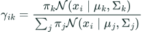
Initialize valid weights, means and covariances. Using the old parameters, compute responsibility γᵢₖ: the posterior fraction of sample i assigned to component k. Each row of responsibilities adds to 1.

\gamma_{ik}=\frac{\pi_k\mathcal N(x_i\mid\mu_k,\Sigma_k)}{\sum_j\pi_j\mathcal N(x_i\mid\mu_j,\Sigma_j)}

Step 3. Use the expected complete-data log likelihood

The “modified” objective in EM is the expectation of the complete-data log likelihood. During this M-step the responsibilities are fixed, so the difficult log of a component sum is replaced by a weighted sum of component log densities.

Q(\theta\mid\theta^{old})=\sum_i\sum_k\gamma_{ik}\left[\log\pi_k+\log\mathcal N(x_i\mid\mu_k,\Sigma_k)\right]

Step 4. M-step: weighted estimates

N_k=\sum_i\gamma_{ik},\quad \pi_k^{new}=\frac{N_k}{N},\quad\mu_k^{new}=\frac{\sum_i\gamma_{ik}x_i}{N_k}

\Sigma_k^{new}=\frac{\sum_i\gamma_{ik}(x_i-\mu_k^{new})(x_i-\mu_k^{new})^T}{N_k}

Repeat E and M until the observed log likelihood changes by less than a chosen tolerance or an iteration limit is reached. EM improves or preserves likelihood under exact steps, but can converge to a local optimum. Try several initializations and avoid singular covariance matrices.

Step 5. Count parameters without inventing the dimension

The question gives K=6, but not the data dimension d or covariance type. For full covariance, each component has d mean entries and d (d+1)/2 independent covariance entries. There are K−1 independent mixture weights.

n_{free}=Kd+K\frac{d(d+1)}2+(K-1)

For a stated one-dimensional assumption: 6 means + 6 variances + 5 independent weights = 17 free parameters. A table may store all 6 weights, giving 18 stored values, but their sum-to-one constraint removes one degree of freedom. With diagonal covariance the general count is 2 Kd+K−1.